Get Unique Values in Excel 2019 and 2016 (No UNIQUE Function)

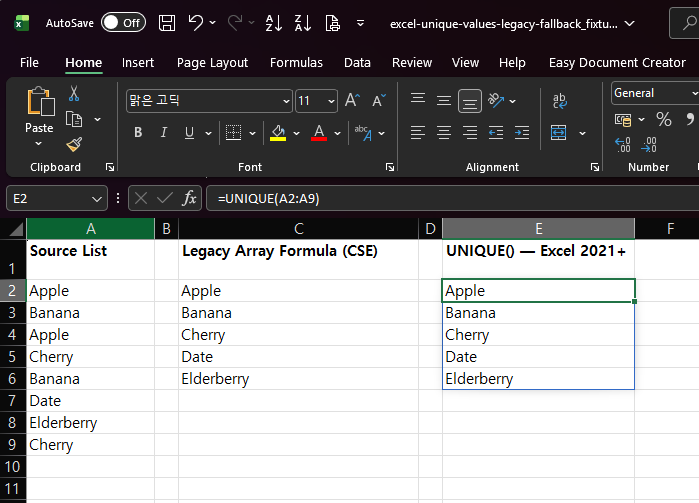
Excel’s UNIQUE() function is the simplest way to pull a list of distinct values from a range — but it isn’t available in every version. If you’re on Excel 2019 or Excel 2016, UNIQUE() will return a #NAME? error, and you’ll need a different approach: a legacy array formula that does the same job without it.

Applies to: UNIQUE() is available in Excel for Microsoft 365, Excel 2024, and Excel 2021. The fallback in this article is for Excel 2019 and Excel 2016, which do not have UNIQUE().

Check Your Version First

Before reaching for the fallback below, confirm you actually need it. Microsoft’s official documentation for UNIQUE() lists Microsoft 365, Excel 2024, and Excel 2021 as supported versions — UNIQUE() works natively in Excel 2021, not just in Microsoft 365. If your formula bar shows #NAME? on Excel 2021, that’s more likely an unrelated account or installation issue than a genuine version gap; it’s worth checking your Microsoft 365/Office installation status before concluding your version doesn’t support it. The fallback below is specifically for Excel 2019 and 2016, where UNIQUE() is genuinely not present. If you want to remove duplicate rows instead of listing distinct values, see our guide on removing duplicates with Power Query.

The Legacy Array Formula

This array formula extracts unique values from a range, in the order they first appear, without UNIQUE():

=IFERROR(INDEX($A$2:$A$9, MATCH(0, COUNTIF($C$1:C1, $A$2:$A$9), 0)), "")

Enter this in the first result cell (for example, C2), and confirm it with Ctrl+Shift+Enter instead of just Enter — this is a legacy array formula (also called a CSE formula), and it will not calculate correctly if entered as a normal formula. Excel will show the formula wrapped in curly braces { } in the formula bar once it’s entered correctly (you don’t type the braces yourself). Then fill it down as far as your data could plausibly have unique values.

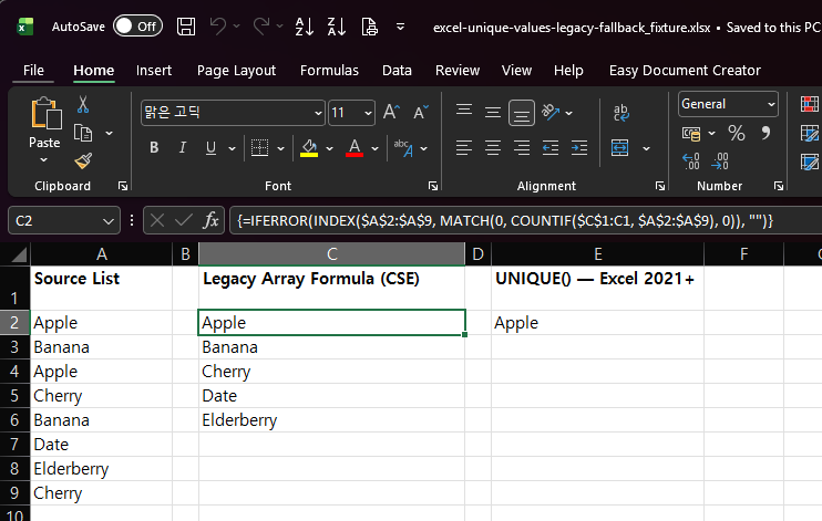
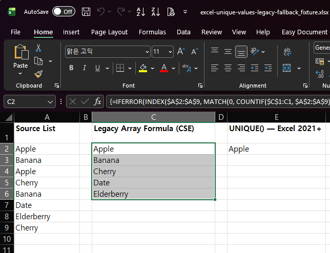
This project directly reproduced this formula in Excel: entering it in C2 and filling down through C6, against a source list in A2:A9 containing Apple, Banana, Apple, Cherry, Banana, Date, Elderberry, Cherry (eight values, with Apple, Banana, and Cherry each appearing twice), produced exactly Apple, Banana, Cherry, Date, Elderberry — the five distinct values, in the order they first appeared in the source list. IFERROR returns "" once every unique value has been extracted, so filling down further than needed doesn’t produce error values in the extra cells.

How the Formula Works

Read it from the outside in:

• COUNTIF($C$1:C1, $A$2:$A$9) — for each value in the source range, counts how many times it has already appeared in the results column so far (the range $C$1:C1 grows as you fill the formula down, since only the first reference is locked with $).
• MATCH(0, ..., 0) — finds the position of the first value in the source range whose count-so-far is 0, meaning it hasn’t been picked yet.
• INDEX($A$2:$A$9, ...) — returns the actual value at that position.
• IFERROR(..., "") — once every value has been picked at least once, MATCH can’t find another 0 and returns an error; IFERROR catches that and shows a blank instead of an error value.

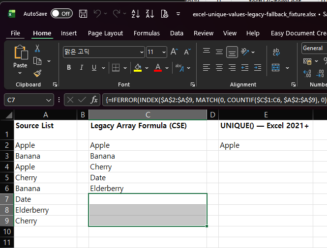
Each row’s formula depends on the results already filled in above it (through the growing $C$1:C1 reference), which is why it has to be entered as an array formula and filled down in order, top to bottom, rather than pasted into a block of cells all at once.

One-line Summary

UNIQUE() works natively in Excel 2021, Excel 2024, and Microsoft 365 — the fallback below is only for Excel 2019 and 2016. There, use =IFERROR(INDEX($A$2:$A$9, MATCH(0, COUNTIF($C$1:C1, $A$2:$A$9), 0)), ""), entered with Ctrl+Shift+Enter and filled down, to extract unique values in the order they first appear.

Sources

• UNIQUE function — Microsoft Support. Backs the version scope: Microsoft 365, Excel 2024, and Excel 2021 support UNIQUE() natively.
• INDEX function, MATCH function, Use the COUNTIF function — Microsoft Support. Back the individual behavior of each function used in the legacy array formula.
• The specific array-formula pattern combining INDEX/MATCH/COUNTIF/IFERROR to extract unique values is a well-known Excel technique, not itself the subject of a single Microsoft documentation page; this project independently reproduced it in Excel against the exact dataset described above (Ctrl+Shift+Enter, filled down C2:C6), confirmed in the Pilot E entry of the project decision log, and the output matched the expected unique list exactly.