Author: CleanSheetHQ Editorial Team

  • Get Unique Values in Excel 2019 and 2016 (No UNIQUE Function)

    Excel’s UNIQUE() function is the simplest way to pull a list of distinct values from a range — but it isn’t available in every version. If you’re on Excel 2019 or Excel 2016, UNIQUE() will return a #NAME? error, and you’ll need a different approach: a legacy array formula that does the same job without it.

    Applies to: UNIQUE() is available in Excel for Microsoft 365, Excel 2024, and Excel 2021. The fallback in this article is for Excel 2019 and Excel 2016, which do not have UNIQUE().

    Check Your Version First

    Before reaching for the fallback below, confirm you actually need it. Microsoft’s official documentation for UNIQUE() lists Microsoft 365, Excel 2024, and Excel 2021 as supported versions — UNIQUE() works natively in Excel 2021, not just in Microsoft 365. If your formula bar shows #NAME? on Excel 2021, that’s more likely an unrelated account or installation issue than a genuine version gap; it’s worth checking your Microsoft 365/Office installation status before concluding your version doesn’t support it. The fallback below is specifically for Excel 2019 and 2016, where UNIQUE() is genuinely not present. If you want to remove duplicate rows instead of listing distinct values, see our guide on removing duplicates with Power Query.
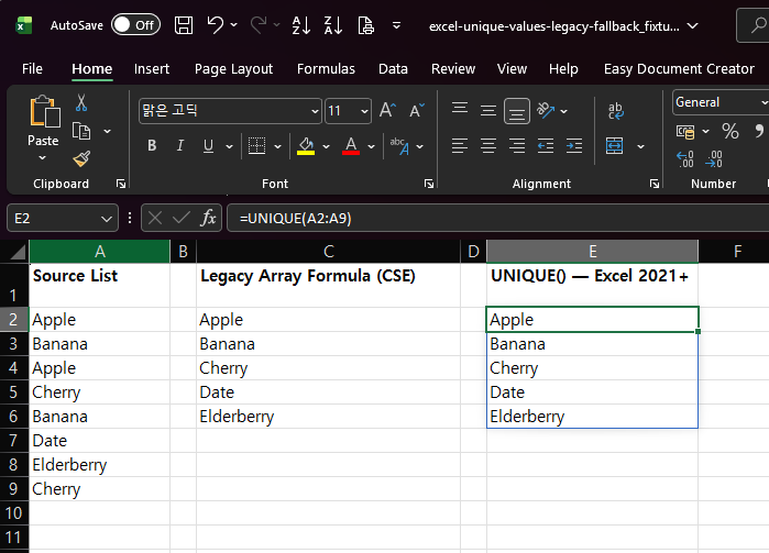
    Excel 2021 sheet where =UNIQUE(A2:A9) in E2 spills Apple, Banana, Cherry, Date and Elderberry next to the legacy formula results

    The Legacy Array Formula

    This array formula extracts unique values from a range, in the order they first appear, without UNIQUE():

    =IFERROR(INDEX($A$2:$A$9, MATCH(0, COUNTIF($C$1:C1, $A$2:$A$9), 0)), "")

    Enter this in the first result cell (for example, C2), and confirm it with Ctrl+Shift+Enter instead of just Enter — this is a legacy array formula (also called a CSE formula), and it will not calculate correctly if entered as a normal formula. Excel will show the formula wrapped in curly braces { } in the formula bar once it’s entered correctly (you don’t type the braces yourself). Then fill it down as far as your data could plausibly have unique values.
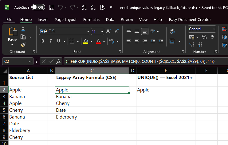
    Excel sheet with the legacy array formula {=IFERROR(INDEX(...MATCH(0,COUNTIF(...),0)),"")} in the formula bar for C2, with Apple in C2 and the source list in column A

    This project directly reproduced this formula in Excel: entering it in C2 and filling down through C6, against a source list in A2:A9 containing Apple, Banana, Apple, Cherry, Banana, Date, Elderberry, Cherry (eight values, with Apple, Banana, and Cherry each appearing twice), produced exactly Apple, Banana, Cherry, Date, Elderberry — the five distinct values, in the order they first appeared in the source list. IFERROR returns "" once every unique value has been extracted, so filling down further than needed doesn’t produce error values in the extra cells.
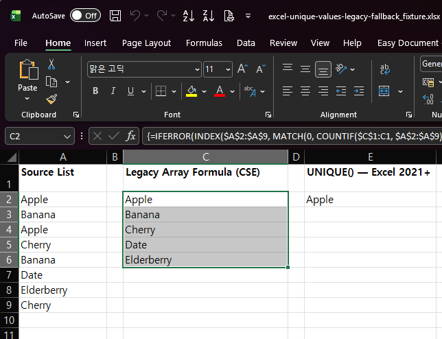
    Excel sheet with C2:C6 selected showing Apple, Banana, Cherry, Date and Elderberry in the order they first appear in the source list

    How the Formula Works

    Read it from the outside in:

    • COUNTIF($C$1:C1, $A$2:$A$9) — for each value in the source range, counts how many times it has already appeared in the results column so far (the range $C$1:C1 grows as you fill the formula down, since only the first reference is locked with $).
    • MATCH(0, ..., 0) — finds the position of the first value in the source range whose count-so-far is 0, meaning it hasn’t been picked yet.
    • INDEX($A$2:$A$9, ...) — returns the actual value at that position.
    • IFERROR(..., "") — once every value has been picked at least once, MATCH can’t find another 0 and returns an error; IFERROR catches that and shows a blank instead of an error value.

    Each row’s formula depends on the results already filled in above it (through the growing $C$1:C1 reference), which is why it has to be entered as an array formula and filled down in order, top to bottom, rather than pasted into a block of cells all at once.
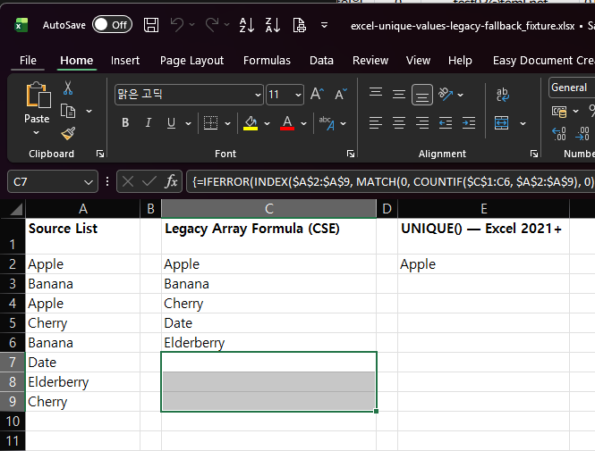
    Excel sheet with the array formula filled down to C9: C2 to C6 show the five unique values and C7 to C9 are blank instead of errors

    One-line Summary

    UNIQUE() works natively in Excel 2021, Excel 2024, and Microsoft 365 — the fallback below is only for Excel 2019 and 2016. There, use =IFERROR(INDEX($A$2:$A$9, MATCH(0, COUNTIF($C$1:C1, $A$2:$A$9), 0)), ""), entered with Ctrl+Shift+Enter and filled down, to extract unique values in the order they first appear.

    Sources

    • UNIQUE function — Microsoft Support. Backs the version scope: Microsoft 365, Excel 2024, and Excel 2021 support UNIQUE() natively.
    • INDEX function, MATCH function, Use the COUNTIF function — Microsoft Support. Back the individual behavior of each function used in the legacy array formula.
    • The specific array-formula pattern combining INDEX/MATCH/COUNTIF/IFERROR to extract unique values is a well-known Excel technique, not itself the subject of a single Microsoft documentation page; this project independently reproduced it in Excel against the exact dataset described above (Ctrl+Shift+Enter, filled down C2:C6), confirmed in the Pilot E entry of the project decision log, and the output matched the expected unique list exactly.
  • Why TRIM Isn’t Removing Non-Breaking Spaces in Excel

    If =TRIM(A2) still leaves extra space in a cell — or two values that look identical still fail an exact-match comparison — the cause is usually a non-breaking space (NBSP, Unicode character U+00A0, decimal code 160), not a regular space. TRIM does not remove it, and one common fix formula can fail depending on your Windows language settings.

    Applies to: all current Excel versions (Excel for Microsoft 365, Excel 2024, Excel 2021, Excel 2019, Excel 2016). The CHAR(160) behavior described below was reproduced specifically on Excel 2021 running on Korean-language Windows — see the scoped explanation in the section below before assuming it applies to your setup.

    Why TRIM Alone Isn’t Enough

    Microsoft’s own documentation for the TRIM function states that the Unicode character set includes an additional space character with decimal value 160 — the non-breaking space commonly used on web pages — and that TRIM by itself does not remove this character. TRIM removes regular ASCII spaces (character code 32) from the start and end of text and collapses multiple spaces between words down to one, but it does not touch character code 160.

    This matters because non-breaking spaces commonly end up in Excel data pasted from web pages, PDFs, or other applications that use them to prevent line breaks. The cell can look completely normal — same font, same visible spacing — while LEN() reports a longer string than expected, or an exact-match formula (=A2=B2) returns FALSE for text that appears identical.

    CLEAN does not solve this either: CLEAN removes the first 32 ASCII control characters (character codes 0–31, non-printing characters like line breaks and tabs), not code 160. A non-breaking space is a printable character, not a control character, so CLEAN has no effect on it.

    TRIM formula failing to remove a non-breaking space in Excel

    The Standard Fix Formula

    The general-purpose pattern for stripping both regular and non-breaking spaces is:

    =TRIM(SUBSTITUTE(CLEAN(A2), UNICHAR(160), " "))

    Read this from the inside out:

    1. CLEAN(A2) strips any non-printing control characters.
    2. SUBSTITUTE(..., UNICHAR(160), " ") replaces every non-breaking space with a regular space.
    3. TRIM(...) then collapses the now-all-regular spaces and trims the ends.
    Full fix formula removing non-breaking spaces and matching expected text length

    A Formula That Can Fail: CHAR(160) vs. UNICHAR(160)

    A common version of this formula uses CHAR(160) instead of UNICHAR(160):

    =TRIM(SUBSTITUTE(A2, CHAR(160), CHAR(32)))

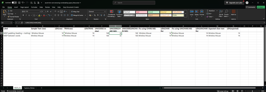
    This project reproduced one specific case where this formula did not fix the problem: on Excel 2021 running on Korean-language Windows. Direct diagnosis in Excel — checking the actual character codes in the source text with UNICODE(MID(...)), then testing =UNICODE(CHAR(160)) directly — showed that on that machine, CHAR(160) did not return the Unicode non-breaking space at all. It returned a regular space (character code 32) instead. Because CHAR(160) was returning the wrong character, SUBSTITUTE had nothing matching to replace, and the non-breaking spaces in the text were left untouched.

    On the tested machine, UNICODE(UNICHAR(160)) returned 160 while UNICODE(CHAR(160)) returned 32. That is why this article uses UNICHAR(160) for the NBSP replacement.

    CHAR(160) returning an unexpected character code on the tested Windows configuration
    UNICHAR(160) correctly returning the non-breaking space on the tested configuration

    This project has confirmed this behavior on one specific configuration (Excel 2021, Korean-language Windows) and has not tested it on other locales. It has not been verified whether this also happens on other non-Western Windows locales, other Excel versions, or other regional settings — that would require separate reproduction on each configuration. Rather than assuming the scope of the issue, the practical takeaway is: verify what CHAR(160) actually returns on your own machine before relying on it (see the check below), and default to UNICHAR(160) in any formula that needs to target the non-breaking space specifically, since it does not depend on this ambiguity.

    How to Check Whether This Affects You

    Before assuming a fix formula worked, verify it rather than trusting that it ran without an error:

    1. Check the actual character code(s) around the suspect space with =UNICODE(MID(A2, n, 1)) for the relevant position n. A non-breaking space returns 160; a regular space returns 32.
    2. Check what your own CHAR(160) actually returns: =UNICODE(CHAR(160)). If this returns 160, CHAR(160) is working correctly as a non-breaking space on your system. If it returns anything other than 160, use UNICHAR(160) instead in any formula that needs to target the non-breaking space.
    3. After applying the fix formula, re-check the result’s length with LEN() against the expected clean length, rather than assuming success because the formula didn’t error.
    UNICODE formula confirming a non-breaking space at code 160

    If the symptom you see is a lookup returning #N/A, see our guide on VLOOKUP or XLOOKUP returning #N/A on values that look identical. If you are cleaning phone numbers copied from a web page, see our guide on standardizing US phone numbers.

    One-line Summary

    TRIM alone does not remove non-breaking spaces (character code 160); use =TRIM(SUBSTITUTE(CLEAN(A2), UNICHAR(160), " ")). On at least one tested configuration (Excel 2021, Korean-language Windows), CHAR(160) returned the wrong character and silently broke a CHAR(160)-based fix formula — check what =UNICODE(CHAR(160)) returns on your own machine, and prefer UNICHAR(160) if you’re unsure.

    Sources

    • TRIM function — Microsoft Support. States that Unicode includes an additional space character (decimal value 160, the non-breaking space used on web pages) and that TRIM by itself does not remove it.
    • UNICHAR function — Microsoft Support. Backs UNICHAR’s behavior of returning the character for a given Unicode code point.
    • CLEAN function — Microsoft Support. Backs the statement that CLEAN removes the first 32 ASCII control characters and does not affect character code 160.
    • The CHAR(160) behavior — returning a regular space (code 32) instead of the non-breaking space on one specific machine (Excel 2021, Korean-language Windows), while UNICHAR(160) correctly returned code 160 on the same machine — was diagnosed and confirmed by this project through direct reproduction in Excel, recorded in the Pilot C entry of the project decision log. This is a project-verified reproduction on one configuration, not a general claim about Windows locales, and it has not been tested on other locales or Excel versions.
  • How to Remove Blank Rows in Excel Without Breaking Your Formulas

    Go To Special > Blanks > Delete Entire Row is the shortcut most people reach for first, but it selects blank cells — not rows that are completely empty. If your range contains partially filled records, that shortcut can delete rows you meant to keep. If another formula explicitly references one of the deleted rows, you can also end up with a #REF! error.

    This guide shows why the shortcut is risky and walks through a safer method that deletes only rows that are fully blank.

    Applies to: Excel for Microsoft 365, Excel 2024, Excel 2021, Excel 2019, and Excel 2016. Both the shortcut and the safer method below use only long-standing Excel features, so the behavior is the same across every version in this list.

    The Standard Shortcut (and Why It’s Risky)

    1. Select the data range you intend to clean.
    2. Press Ctrl+G, click Special, choose Blanks, then click OK.
    3. Excel selects every blank cell in that range.
    4. If you then choose Delete > Entire Row, every row that contains one of those selected blank cells gets deleted — not just rows that are entirely empty.

    That last step is the trap: a row with just one missing field looks nothing like a “blank row” to the person cleaning the data, but Excel treats it the same way once any cell in it is selected as blank.

    Excel Go To Special dialog box with the Blanks option selected

    Why Partially Blank Rows Can Disappear

    Suppose a customer list contains:

    • a row that is completely blank,
    • a record for Bob with a missing phone number,
    • a record for Dave with a missing email address.

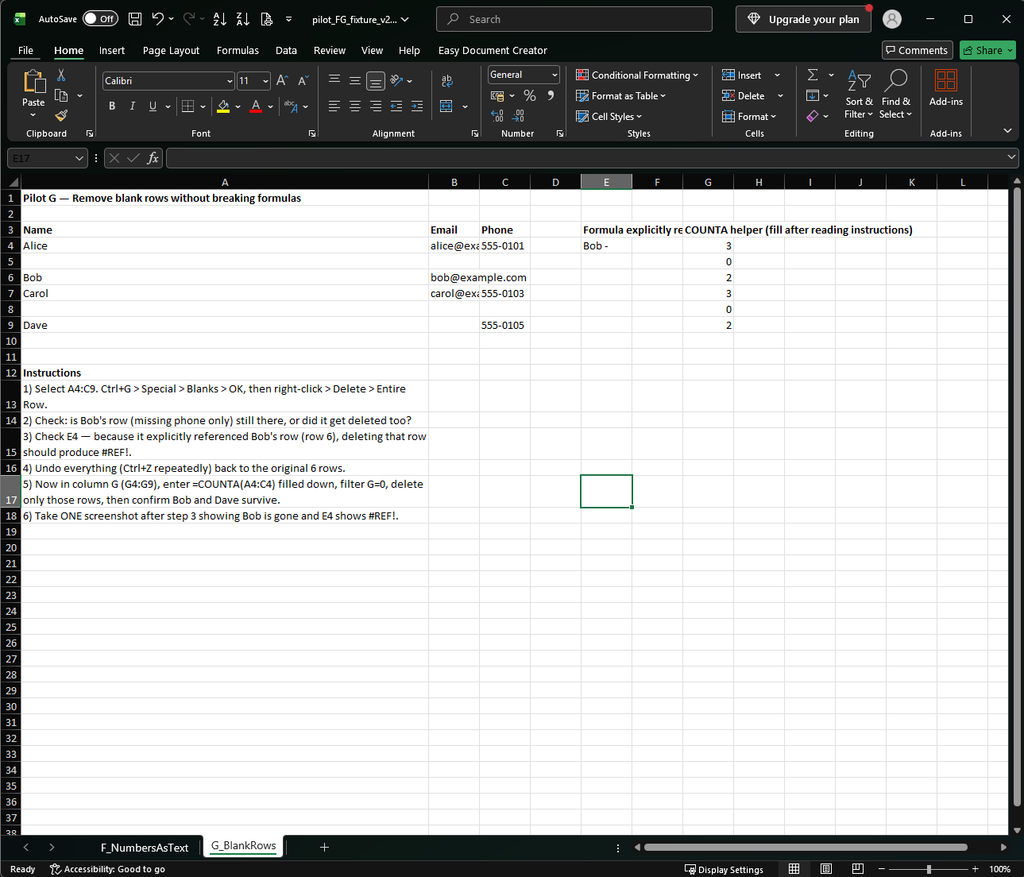
    Bob and Dave are not blank records — they are incomplete records. But Go To Special > Blanks selects Bob’s empty phone cell and Dave’s empty email cell right alongside the cells in the truly blank row. Delete entire rows from that selection, and Bob and Dave can be removed along with the actual blank rows.

    That’s a data-loss problem on its own, before any formula is even involved.

    Excel showing partially filled rows and fully blank rows selected together by Go To Special Blanks

    If your report prints a group label only on the first row, see our guide on filling blank cells with the value above.

    When #REF! Shows Up

    Microsoft documents #REF! as the error Excel shows when a formula’s cell reference is no longer valid — most often because the referenced cells, rows, or columns were deleted. Deleting rows doesn’t automatically break every formula in a sheet; Excel adjusts many range references on its own. The failure case is clearest when a formula explicitly names a row that then gets deleted by the blanks shortcut. In that situation, the formula returns #REF! because the exact cell it pointed to no longer exists.

    If you catch the mistake right away, Ctrl+Z is the fastest way to recover before doing anything else.

    Excel formula showing a #REF! error after the row it referenced was deleted

    The Safer Method: Delete Only Fully Blank Rows

    Add a helper column that counts how many non-empty cells each record has, using COUNTA.

    For a three-column dataset in columns A:C, starting at row 4:

    =COUNTA(A4:C4)

    Fill the formula down the full range. Then read the result:

    • 0 — the row is completely blank across the checked columns.
    • 1 or more — at least one field has data, so the row is incomplete, not blank, and shouldn’t be deleted by this pass.
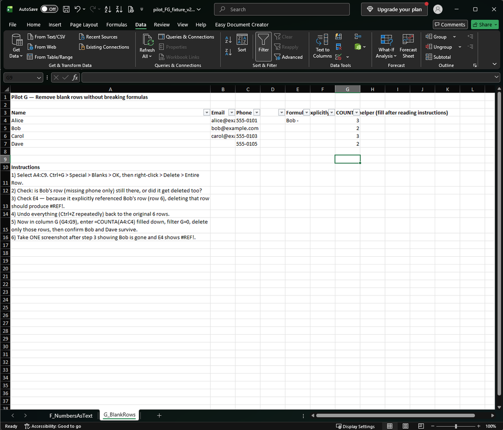
    Excel COUNTA helper column distinguishing fully blank rows (0) from partially filled rows (1 or more)

    Now clean up safely:

    1. Filter the helper column to 0.
    2. Delete only the visible, fully-blank rows.
    3. Clear the filter.
    4. Remove the helper column once you’re done.

    This keeps Bob’s and Dave’s partially filled records intact while still clearing out the rows that are genuinely empty.

    Excel spreadsheet after safely removing only fully blank rows, keeping partially filled records intact

    Formula Design Also Reduces the Risk

    Beyond the helper-column cleanup itself, how you write formulas in the first place affects how much a future row deletion can break. A continuous range adjusts automatically when rows inside it are removed; a formula built from a list of individual cell references does not adjust the same way. For example:

    =SUM(B2:D2)

    is generally more resilient to structural edits than:

    =SUM(B2,C2,D2)

    This is a separate safeguard from the COUNTA helper — the helper stops you from deleting the wrong rows in the first place, while range-based formulas reduce how much damage a future structural change can cause even when it does happen.

    One-line Summary

    Go To Special > Blanks selects blank cells, so deleting entire rows from that selection can remove partially filled records along with truly empty ones — and can break any formula that explicitly references a deleted row with #REF!. If you only want rows that are completely empty, filter on a COUNTA(...)=0 helper column first.

    Sources

    • Find and select cells that meet specific conditions in Excel — Microsoft Support. Documents the Go To Special > Blanks behavior this article builds on.
    • How to correct a #REF! error — Microsoft Support. Backs the explanation of when and why #REF! appears after a deletion.
    • COUNTA function — Microsoft Support. Reference for the COUNTA helper-column method.
    • Range-vs-list formula resilience and the exact #REF! reproduction (a formula explicitly referencing a row deleted by the Blanks shortcut) were confirmed by this project’s own reproduction in Excel, recorded in the Pilot G entry of the project decision log and this article’s QA package — not solely from the official pages above.
  • How to Convert Numbers Stored as Text in Excel (4 Bulk Methods)

    If a column of numbers is left-aligned, shows a small green triangle in the corner of each cell, or calculations such as SUM ignore the values, Excel may be treating those values as text rather than numbers. This is common after importing data from CSV files, databases, or copy-pasting from a website.

    Here are four ways to fix it in bulk, plus a hidden-character case that can make a value look like it’s still text after you’ve tried one of them.

    Applies to: Excel for Microsoft 365, Excel 2024, Excel 2021, Excel 2019, and Excel 2016. All four methods below use only long-standing Excel features (no new dynamic-array functions), so they work the same way across every version in this list.

    Method 1: Error Checking Button (fastest when available)

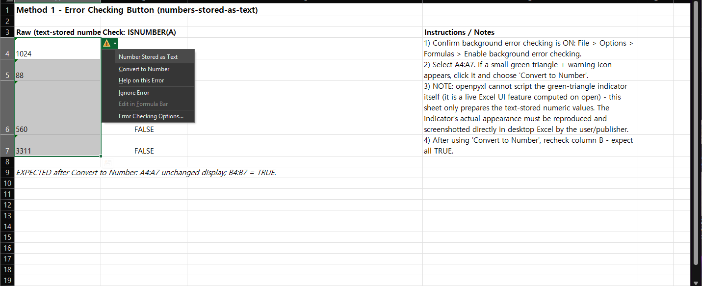
    If Excel’s background error checking is on, cells with text-stored numbers can show a small green triangle in the top-left corner.

    1. Select the cells you want to convert.
    2. Click the warning icon that appears next to the selection.
    3. Choose Convert to Number.

    If you do not see the warning icon, background error checking may be disabled under File > Options > Formulas > Enable background error checking.

    Excel warning icon showing the Convert to Number option for cells with numbers stored as text

    Method 2: Paste Special → Multiply

    This method works even when the error-checking indicator is unavailable:

    1. Type 1 in an empty cell.
    2. Copy that cell.
    3. Select the range containing numbers stored as text.
    4. Open Paste Special.
    5. Choose Multiply under Operation, then click OK.

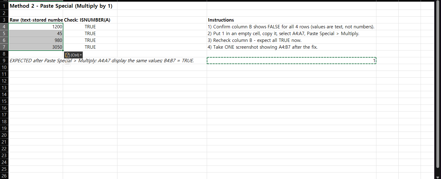
    Multiplying by 1 forces text-formatted numeric values to become numeric values while leaving their displayed numbers unchanged.

    Excel Paste Special dialog with Multiply selected, converting text-stored numbers to real numbers

    Method 3: VALUE() Helper Column

    For mixed or messy imports, a helper column makes the conversion visible and easier to audit:

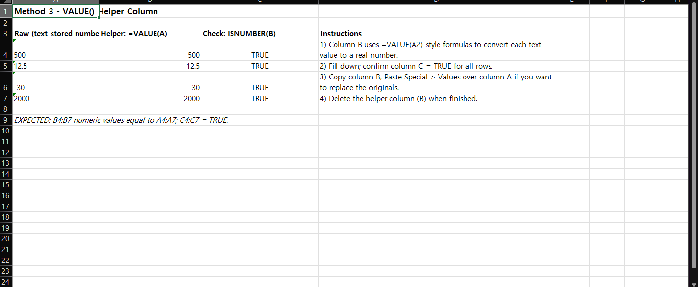
    1. In a new column, enter =VALUE(A2) and adjust the reference as needed.
    2. Fill the formula down.
    3. Copy the converted results.
    4. Use Paste Special > Values if you want to replace the original text values.
    5. Remove the helper column when finished.

    VALUE converts text that Excel recognizes as a valid number, date, or time into a numeric value.

    Excel helper column using the VALUE function to convert text-stored numbers

    Method 4: Text to Columns

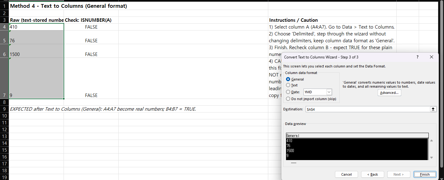
    Text to Columns can also cause Excel to reinterpret simple numeric text using the General column format.

    1. Select the column containing the text-stored numbers.
    2. Go to Data > Text to Columns.
    3. Keep the column format as General.
    4. Finish the wizard.

    Use this method carefully if the source contains leading zeros, long identifiers, dates, or mixed text-and-number values, because automatic conversion may change how those values are represented.

    Excel Text to Columns wizard with General column format selected

    If Conversion Still Fails, Check for Hidden Characters

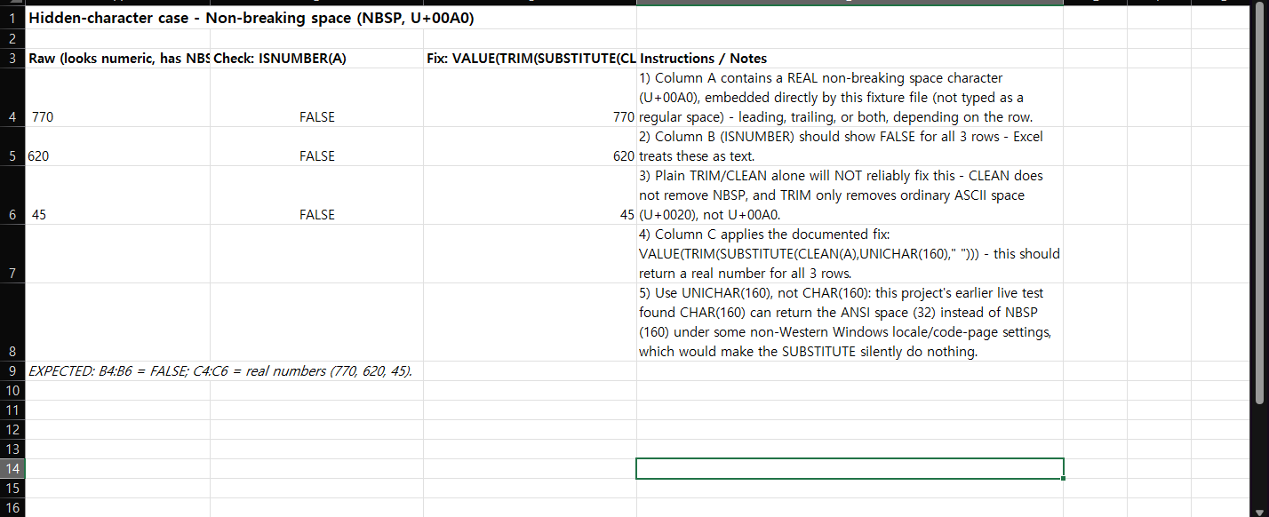
    A value can look numeric while still containing a hidden character, such as a non-breaking space (NBSP, Unicode character 160) left over from a web copy-paste or an export from another system. When a value contains one, the methods above may not convert it, because Excel still sees a text string rather than a clean number.

    TRIM removes ordinary spaces (the character you get from pressing the spacebar, code 32) and collapses multiple spaces between words down to one — but by itself it does not remove the non-breaking space character. CLEAN removes the first 32 nonprinting ASCII control characters (codes 0–31); the non-breaking space falls outside that range, so CLEAN does not address it either. In other words, TRIM and CLEAN are each scoped to a different kind of unwanted character, and neither is designed to target a literal U+00A0.

    For a closer look at this, see our guide on why TRIM isn’t removing non-breaking spaces.

    To target the non-breaking space specifically, use UNICHAR(160), which returns the Unicode character for code point 160 — the non-breaking space — so it can be matched and replaced explicitly:

    =VALUE(TRIM(SUBSTITUTE(CLEAN(A2),UNICHAR(160)," ")))

    For readability on smaller screens, here is the same formula wrapped across lines (the single-line version above is the one to copy):

    =VALUE(
      TRIM(
        SUBSTITUTE(
          CLEAN(A2),
          UNICHAR(160),
          " "
        )
      )
    )

    This formula uses CLEAN to strip ordinary control characters, SUBSTITUTE with UNICHAR(160) to swap the literal non-breaking space for a regular space, TRIM to clean up the result, and VALUE to convert the cleaned text into a number.

    Excel formula using UNICHAR(160) to fix numbers stored as text with a hidden non-breaking space

    Which Version of Excel Do You Need?

    All five techniques in this article — the four bulk-conversion methods and the UNICHAR fix — work in Microsoft 365, Excel 2024, Excel 2021, Excel 2019, and Excel 2016. None of them depend on newer dynamic-array functions like UNIQUE, FILTER, or TEXTSPLIT, so there is no version-specific fallback needed here.

    One-line Summary

    For a quick one-time fix, use Convert to Number or Paste Special > Multiply. For mixed imported data, use a helper formula such as VALUE() so you can see which rows converted successfully before replacing the source values. If a value still won’t convert, check for a hidden non-breaking space and use the UNICHAR(160) formula above.

    Sources

    • Convert numbers stored as text to numbers in Excel — Microsoft Support. Backs Method 1 (error-checking indicator, Convert to Number) and Method 3 (VALUE as a helper-column method).
    • Fix text-formatted numbers by applying a number format — Microsoft Support. Backs Method 2 (Paste Special with Multiply).
    • VALUE function — Microsoft Support. Reference for the VALUE function used in Method 3 and in the hidden-character formula.
    • TRIM function — Microsoft Support. Explicitly documents the non-breaking space (decimal 160) and states that TRIM alone does not remove it — the basis for the “Check for Hidden Characters” section.
    • CLEAN function — Microsoft Support. Documents that CLEAN removes only the first 32 nonprinting ASCII control characters, which do not include the non-breaking space.
    • UNICHAR function — Microsoft Support. Reference for UNICHAR, which returns the Unicode character for a given code point (160 for the non-breaking space).
    • Split text into different columns with the Convert Text to Columns Wizard — Microsoft Support. General reference for the Text to Columns wizard used in Method 4. Note: this page does not document the specific behavior of “General” format reinterpreting text-stored numbers — that claim rests on this project’s own reproduction in Excel, not on this official page.