Import Long Numbers in Excel Without Scientific Notation or Lost Digits

You open a CSV in Excel and a 16-digit tracking number turns into 1.23457E+15. A 12-digit reference number turns into 1.23457E+11. Both look like the same problem, but they are not. Excel only changed how the 12-digit number is displayed. For the 16-digit number, Excel also changed the stored value.

This guide explains how to stop Excel scientific notation on long numbers by importing the CSV with Data > From Text/CSV and setting those columns to Text before the data reaches the worksheet. It also shows why a number that has already lost digits cannot be repaired inside Excel, so the original file is what you need.

Applies to: Microsoft documents the 15-digit limit, the leading-zeros and large-number behavior, and the From Text/CSV import for Excel for Microsoft 365, Excel 2024, Excel 2021, Excel 2019, and Excel 2016. Tested in the Excel desktop app with an English interface on Korean-language Windows. We did not test other Excel versions, so menu names may look slightly different there.

The screenshots use a small made-up CSV with a 16-digit tracking_no column (1234567890123456, 9876543210987654, and so on) and a 12-digit ref_no column (123456789012, 987654321098, and so on).

What Goes Wrong When You Double-Click a CSV

When you open a .csv file directly, Excel applies its default format settings to each column. For long digit strings, that means they are read as numbers.

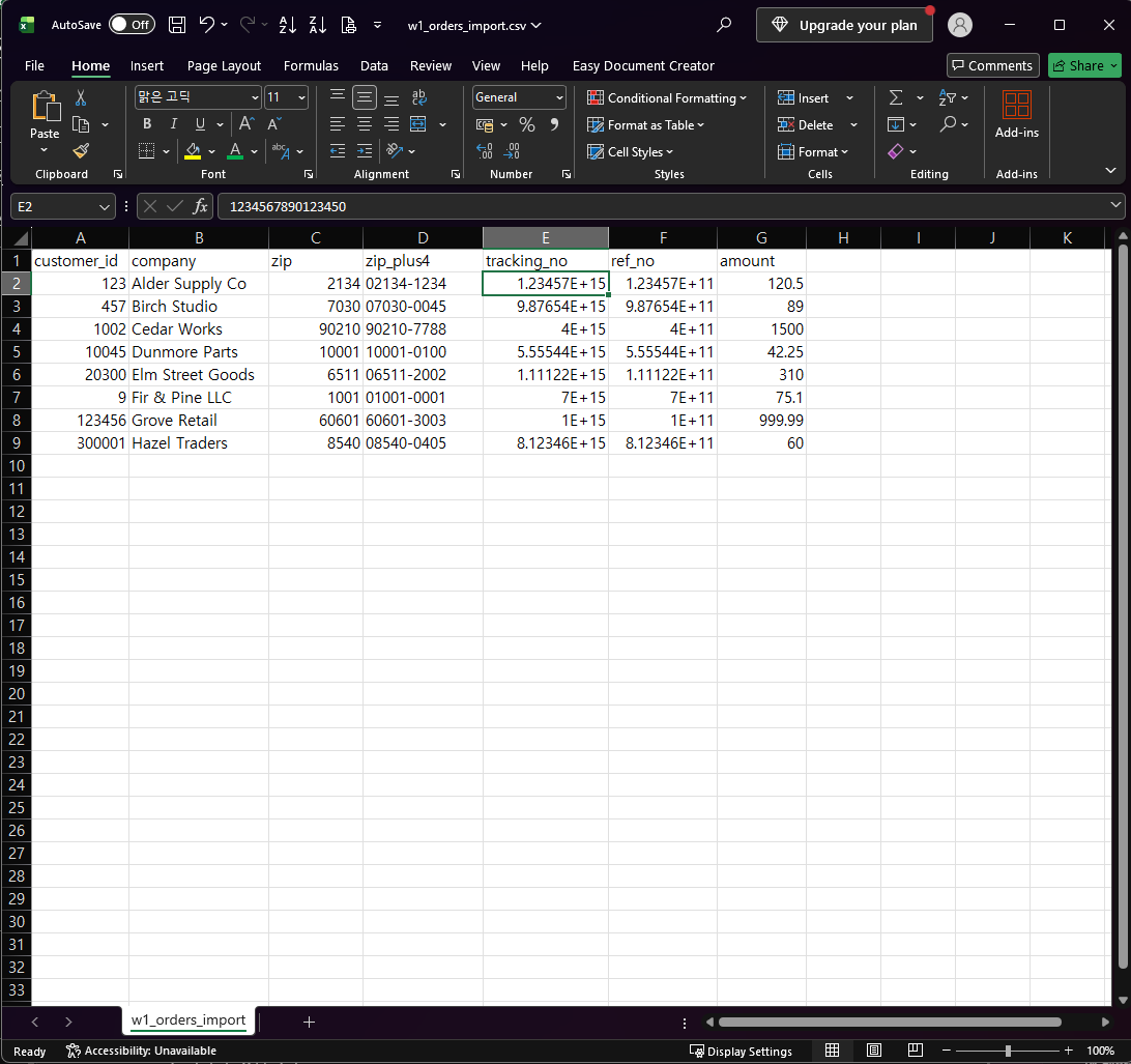
In our test, tracking_no appeared as 1.23457E+15 and ref_no as 1.23457E+11. Click cell E2 and look at the formula bar. The CSV contains 1234567890123456, but the formula bar shows 1234567890123450. The last digit has already changed from 6 to 0.

Two Different Problems: Display vs. Lost Digits

We selected both columns, applied the Number format with 0 decimal places, and widened the columns.

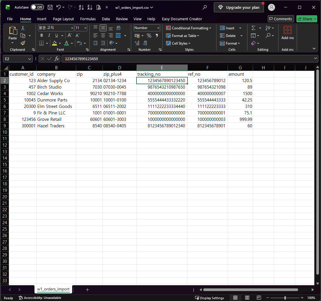
The two columns behaved differently:

Column	In the CSV	In Excel after Number format	What it means
ref_no (12 digits)	123456789012	123456789012	Display problem only. The value was kept.
tracking_no (16 digits)	1234567890123456	1234567890123450	The stored value changed.

Across all 8 rows of our test file, the 12-digit ref_no values matched the CSV exactly once we applied the number format, and the 16-digit tracking_no values had their last digit replaced with 0 in all 8 rows. (We checked the formula bar only for E2, so the other rows are based on the values shown in the cells.)

This matches what Microsoft documents: Excel keeps a maximum of 15 significant digits, and for numbers with 16 or more digits, the digits after the 15th become zeros. A 12-digit number is within that limit, so Excel kept it. Changing the number format afterward did not bring the last digit of tracking_no back, and Microsoft says the same about formats applied after the fact. We tested only the Number format.

The Safest Method: Import With Data > From Text/CSV

This is the same method as in our guide to keeping leading zeros in ZIP codes and ID numbers, applied to long numbers.

1. Do not double-click the CSV. Open a new blank workbook in Excel instead.
2. Go to the Data tab, click From Text/CSV, select your file, and click Import.
3. In the preview window, click Transform Data. This opens the Power Query Editor.
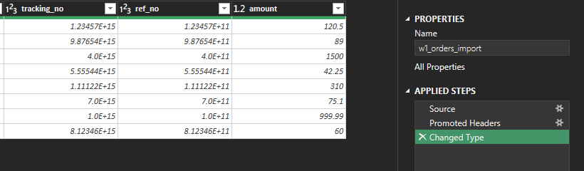
4. In the Applied Steps pane on the right, find the Changed Type step that Excel added automatically. In our test it had set tracking_no and ref_no to whole numbers (the 123 icon in the column header), and the values already appeared as 1.23457E+15 and 1.23457E+11. We deleted this step before setting Text. Click the X next to Changed Type to delete it.

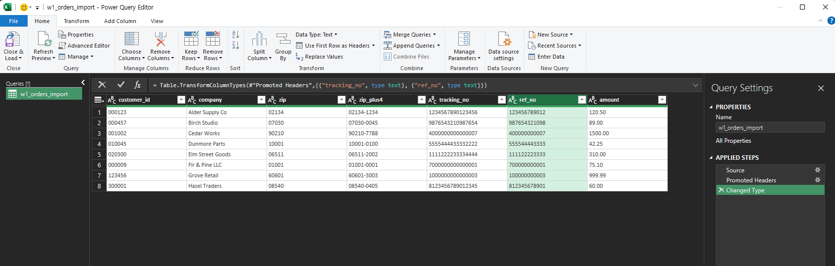
5. Click the data type icon at the left of the tracking_no column header and choose Text. Repeat for ref_no. Both columns should show the ABC icon and the full values, such as 1234567890123456 and 123456789012.

6. On the Home tab, click Close & Load.

Select E2 in the new worksheet. The formula bar should show 1234567890123456.

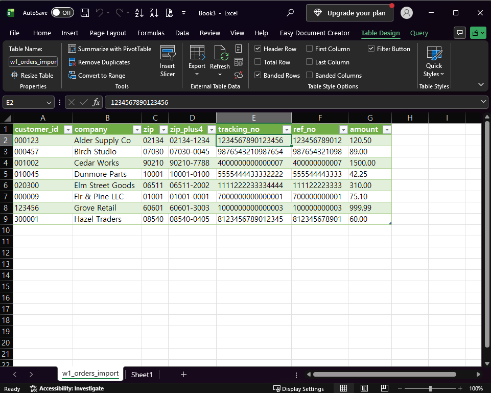
In our test, all 8 tracking_no values and all 8 ref_no values matched the original CSV. Keep identifiers such as tracking numbers, account numbers, and card-style codes as Text. If you ever need to calculate with a column, convert it to numbers first. Be aware that a number with more than 15 digits would lose digits at that point, so do not convert identifiers like these.

If You Already Opened the CSV the Usual Way

Once Excel has converted a 16-digit number, the cell no longer contains the original last digit. The formula bar in the first screenshot shows 1234567890123450, and reformatting the cell does not change it. Microsoft’s guidance is to use the Text format for codes with 16 or more digits.

Go back to the original file:

1. Close the workbook without saving.
2. Re-import the original CSV with the steps in the previous section.

In our test we closed the double-clicked file without saving and the original CSV was unchanged. The cells hold the changed values, so anything you save from them cannot contain the lost digits. We did not test what happens when you save the workbook over the original, so keep the original file untouched. If you saved the converted data over the only copy of the CSV, check file history, backups, or the system that produced the file. Do not try to guess the missing digits from the worksheet.

A 12-digit number that only looks like 1.23457E+11 is different. Its value was kept, and the number format changes how it is displayed. If you still have the original CSV, importing it as Text is the cleaner path for both columns.

Which Version of Excel Do You Need?

Microsoft lists Excel for Microsoft 365, Excel 2024, Excel 2021, Excel 2019, and Excel 2016 as applying to the source pages below. This guide uses no new functions. We tested only one desktop Excel build (English interface, Korean-language Windows), so button names in other versions may differ slightly.

One-line Summary

Excel keeps only 15 significant digits, so do not double-click a CSV that contains 16-digit numbers. Import it with Data > From Text/CSV, click Transform Data, delete the automatic Changed Type step, set those columns to Text, and click Close & Load. If the digits are already zeroed out, re-import the original file.

Sources

• Keeping leading zeros and large numbers — Microsoft Support. Backs the 15-significant-digit limit, the digits after the 15th becoming zeros, the advice to use Text for numbers with 16 or more digits, and that applying a format afterward does not change what was already entered.
• Excel specifications and limits — Microsoft Support. Lists number precision as 15 digits in the calculation specifications.
• Import or export text (.txt or .csv) files — Microsoft Support. Backs the Data > From Text/CSV path and the statement that opening a .csv directly applies Excel’s default format settings.
• Note: the 1.23457E+15 and 1.23457E+11 displays, the 1234567890123450 formula bar value, the 8/8 and 8/8 row comparison, and the full values after Close & Load come from our own reproduction in the Excel desktop app, not from these pages.