Category: Data Cleanup

  • How to Exclude Hidden Rows, Hidden Columns and Filtered Rows When Saving CSV in Excel

    You hid a few rows, filtered a list, or hid a column such as an internal cost, and then saved the sheet as a CSV to send to someone. Did the hidden parts go into the file? We tested three cases in Excel, read the bytes of every file we saved, and tried one way to leave the hidden parts out of each.

    Short answer from our test: saved as they were, all three cases wrote every row and column into the CSV. To leave them out, we copied only the visible cells to a new workbook and saved that. The steps differ a little between the three cases, and we list exactly what worked.

    Tested in: Excel 2021 desktop (Version 2608) with an English interface, on Windows with Korean regional settings (list separator ,, decimal point .). Everything below describes what happened on that one setup. We did not test other Excel versions, other regional settings, or Mac, and results may differ there.

    Our Test Sheets

    We made three small workbooks with a script. Each has the same ten data rows in columns A to E:

    On a phone, you can swipe this table sideways to see all the columns.

    idcustomerregionstatusinternal_cost
    1Acme CoEastopen110
    2Bolt LtdWestclosed220
    3Cobalt IncEastopen330
    4Delta LLCWestopen440
    5Echo GmbHNorthclosed550
    6Fjord ASEastopen660
    7Gamma SAWestclosed770
    8Helix BVNorthopen880
    9Iris OyEastopen990
    10Juno PtyWestclosed1010
    • Workbook A, hidden rows: we hid the rows for id 3 and id 7.
    • Workbook B, filtered rows: we filtered the region column to show only West, so ids 2, 4, 7 and 10 stayed visible.
    • Workbook C, hidden column: we hid column E, internal_cost.

    We kept these workbooks as they were. Every CSV below was saved under a new file name as “CSV UTF-8 (Comma delimited)”. We did not test the other CSV format here; our byte-level comparison of the two CSV save options covers how they differ.

    Step 1: Save As They Are

    We opened each workbook and used File > Save As without changing anything. The result was the same in all three cases: the file had a header line and ten data lines, and every line had all five fields, including the rows we hid or filtered out and the hidden internal_cost column. The three files were byte-for-byte identical to each other.

    So in our test, hiding a row, filtering it out, or hiding a column changed what Excel showed, not what it wrote. Our earlier post on what a CSV holds compared with what the cells display mentions hidden rows and columns in two short bullets; this post tests the three cases on their own.

    Hidden Rows: Copy the Visible Cells Only
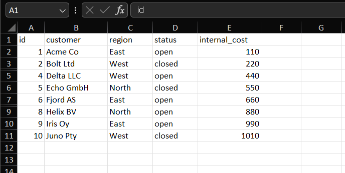
    Excel sheet with ids 3 and 7 hidden, so the row numbers skip and only ids 1, 2, 4, 5, 6, 8, 9 and 10 are visible
    Workbook A: the rows for ids 3 and 7 are hidden, and the row numbers skip over them.

    The screenshot shows workbook A with ids 3 and 7 hidden. The row numbers skip where the hidden rows are.

    We first tried the plain way. We pressed Ctrl+A, then Ctrl+C, opened a new workbook with Ctrl+N, pasted with Ctrl+V and saved that as a CSV. The file still had all ten rows. In our test, an ordinary copy of manually hidden rows took them along.

    What worked:

    1. Press Ctrl+A to select the sheet.
    2. Press Alt+; (Alt and the semicolon key). This is the shortcut for Select Visible Cells.
    3. Press Ctrl+C.
    4. Press Ctrl+N for a new workbook, then Ctrl+V.
    5. Use File > Save As and choose a CSV format, with a new file name.

    The CSV had the header and eight data rows: ids 1, 2, 4, 5, 6, 8, 9 and 10. Ids 3 and 7 were not in the file, and the values in the other rows were unchanged.

    Filtered Rows: Copy and Paste the Filtered List
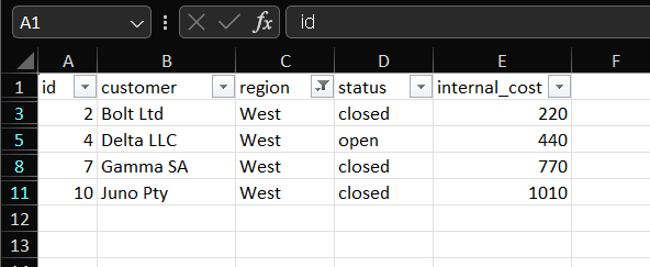
    Excel sheet with a filter on the region column showing only the West rows with ids 2, 4, 7 and 10
    Workbook B: the region filter is set to West, so only ids 2, 4, 7 and 10 are visible.

    The screenshot shows workbook B with the region filter set to West. The filter button on the region column shows that a filter is on.

    Here the plain copy was enough. We pressed Ctrl+A, Ctrl+C, opened a new workbook, pasted, and saved as a CSV. The file had the header and four data rows: ids 2, 4, 7 and 10. The rows hidden by the filter were not in the file.

    We did not try Alt+; on the filtered list, so we cannot say whether it changes anything there. We also do not know why a plain copy left out the filtered rows but not the manually hidden ones. We only saw that it did.

    Hidden Columns: Copy the Visible Cells Only
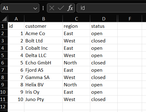
    Excel sheet whose column letters jump from D to F because column E, internal_cost, is hidden
    Workbook C: the column letters jump from D to F because column E is hidden.

    The screenshot shows workbook C. The column letters jump from D to F because column E is hidden.

    A plain copy and paste into a new workbook took the hidden column along: the new workbook had five columns, and the CSV saved from it still had internal_cost. With Select Visible Cells, it did not:

    1. Press Ctrl+A to select the sheet.
    2. Press Alt+;.
    3. Press Ctrl+C.
    4. Press Ctrl+N, then Ctrl+V.
    5. Use File > Save As and choose a CSV format, with a new file name.

    The CSV had four fields on every line, id,customer,region,status, and ten data rows. The internal_cost values were not in the file.

    How We Checked the Results

    For each file we looked at the saved bytes outside Excel, not only at the sheet:

    CaseWay we savedData rows (header line not counted)Fields per line
    Hidden rowsAs is105
    Hidden rowsPlain copy to a new workbook105
    Hidden rowsSelect Visible Cells, copy to a new workbook85
    Filtered rowsAs is105
    Filtered rowsPlain copy to a new workbook45
    Hidden columnAs is105
    Hidden columnPlain copy to a new workbook105
    Hidden columnSelect Visible Cells, copy to a new workbook104

    For the files that used a workaround, we compared the remaining values with the source: nothing visible went missing, and none of the hidden ids or the internal_cost values appeared.

    How We Would Use This

    • Do not trust a hidden or filtered row to stay out of a CSV. In our test, only copying to a new workbook did that.
    • For manually hidden rows or hidden columns, use Alt+; before copying. For a filtered list, a plain copy worked in our test.
    • Before you share or upload the CSV, open it in a text editor or reopen it, and check that the rows or columns you meant to leave out are not in it, and that the ones you wanted are. We checked this by comparing the ids and column names in each saved file.
    • Keep the original workbook, and save the CSV under a new file name.

    Things to Know

    • Scope. Everything above comes from three small test workbooks on Excel 2021 (Version 2608) with Korean regional settings and a comma list separator. Other Excel versions, other regional settings and Mac may behave differently.
    • Not tested. Hiding rows and columns in the same sheet, grouped (outline) rows and columns, Excel tables and slicers, merged cells in the copied range, formulas that refer to hidden cells, using Alt+; on a filtered list, deleting the hidden column instead of copying, Power Query, macros, and Excel for the web.
    • Unconfirmed. Why a plain copy kept manually hidden rows and columns but not filtered rows.

    One-line Summary

    In our Excel 2021 test, hidden rows, filtered-out rows and a hidden column were all written to the CSV when we saved as is, and copying the visible cells to a new workbook before saving left them out.

    Sources

    The screenshots and behavior described as “we saw” come from our own test in Excel 2021 on one setup. We did not rely on Microsoft documentation for the results above.
  • Excel Save as CSV: Displayed Values, Formulas and Long Numbers

    A cell in Excel can show one thing and hold another: $1,234.50 on screen, 1234.5 in the formula bar. When you save the sheet as a CSV, which one ends up in the file? We saved a small test sheet in Excel, read the bytes of the files, and reopened one of them to see what survived.

    This guide shows the cells we tested, what Excel wrote for each one, what changed when we turned on Show Formulas first, and what happened to a 16-digit number.

    Tested in: Excel 2021 desktop (Version 2608) with an English interface, on Windows with Korean regional settings (list separator ,, decimal point .). Everything below describes what happened on that one setup. We did not test other Excel versions, other regional settings, or Mac, and results may differ there.

    Our Test Sheet

    We created a workbook with a script, with 19 data rows. These are the rows that matter most for this question:

    On a phone, you can swipe this table sideways to see all the columns.

    CellWhat we put inFormatShown in Excel
    C21234.5$#,##0.00$1,234.50
    C33.141590.003.14
    C40.2560.0%25.6%
    C5a datedd/mm/yyyy05-03-2026
    C61230000000123
    C7text 00123text00123
    C81234567890123456General1.23457E+15
    C9text 1234567890123456text1234567890123456
    C10123456789012345601234567890123460
    C11formula =1234.5*2General2469
    C13formula =NA()General#N/A

    On our PC, the slash in the date format dd/mm/yyyy was displayed as a hyphen. The sheet also has a few cells for hidden rows and columns, a merged range, a narrow column, and euro amounts; we cover those near the end.

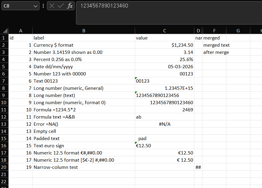
    Excel test sheet in normal view with cell C8 selected and its formula bar showing 1234567890123460, while the cell displays 1.23457E+15
    The test sheet in normal view: C8 displays 1.23457E+15, and its formula bar shows 1234567890123460.

    The screenshot shows cell C8 selected. Its formula bar reads 1234567890123460, even though our script wrote 1234567890123456 into the file. We did not look into why. We kept this workbook as it was and saved new files from it.

    Saving the Sheet as CSV

    We used File > Save As and saved the sheet twice under new file names, once as “CSV UTF-8 (Comma delimited)” and once as “CSV (Comma delimited)”. Excel did not show a warning dialog for either save. After each save, a yellow “POSSIBLE DATA LOSS” bar appeared above the sheet, saying some features might be lost in the comma-delimited format.

    For the value cells in the table above, the two files had the same text. The differences were the BOM at the start of the UTF-8 file and the euro sign bytes, which we describe below. If you are choosing between the two formats, our byte-level comparison of both save options covers those differences.

    What Excel Wrote

    We looked at the bytes of both files outside Excel. Here is what each cell became:

    CellIn the saved CSV
    C2"$1,234.50" (quoted because of the comma)
    C33.14
    C425.6%
    C505-03-2026
    C600123
    C700123
    C112469
    C13#N/A

    In every one of these, the file holds what the cell displayed: the dollar sign and the thousands comma, the two decimals, the percent sign, the leading zeros from the 00000 format, and the date as it appeared. The number behind C3, 3.14159, is not in the file. In our test this matched Microsoft’s description that the format saves values as displayed (see Sources).

    Formula cells were saved as their results, not as formulas: =1234.5*2 became 2469. A cell with padding spaces, pad , kept its spaces. Each row ended with a carriage return and a line feed (0D 0A).

    Long Numbers: In Excel, Then in the File

    We want to keep two things apart here: the value Excel held before saving, and the text in the saved file. We tried three cells.

    On a phone, you can swipe this table sideways to see all the columns.

    CellWhat our script wroteFormula bar in ExcelSaved CSV
    C8, number, General123456789012345612345678901234601.23457E+15
    C10, number, format 0123456789012345612345678901234601234567890123460
    C9, text123456789012345612345678901234561234567890123456

    The General-format cell was saved in scientific notation, because that is what the cell displayed. The other digits are not in the file. The cell with the 0 format displayed all 16 digits, so the file has them, but the last digit is the 0 that Excel held, not the 6 our script wrote. The text cell kept all 16 digits exactly.

    If you need every digit of a long ID in the CSV, our test points to keeping it in a text cell before you save. Our earlier posts on long numbers turning into scientific notation and on leading zeros in CSV imports cover the opening side of the same problem.

    Show Formulas Changes What Is Saved

    We pressed Ctrl and the grave accent key (the key to the left of 1) to turn on Show Formulas, then saved the same sheet as “CSV UTF-8 (Comma delimited)” under another name. We did not try the other CSV format in this mode.

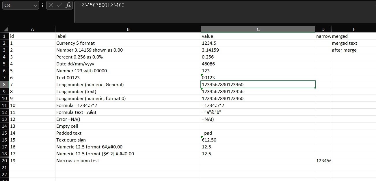
    The same Excel test sheet with Show Formulas on, showing raw values such as 1234.5, 0.256 and 46086 and formulas such as =1234.5*2 instead of formatted results
    The same sheet with Show Formulas on: raw values and formulas instead of formatted results.

    Tap the image to view it at full size.

    The file followed the screen again, and now the screen showed formulas and raw values:

    • Formula cells were saved as text: =1234.5*2, ="a"&"b" (written as "=""a""&""b"""), and =NA().
    • Number formats were gone. C2 was 1234.5, C3 was 3.14159, C4 was 0.256, the date was 46086, and the 00000 cell was 123.
    • The long number in General format was 1234567890123460, with all its digits, because the cell no longer showed scientific notation.
    • Text cells, 00123 and the long number text, were unchanged.

    If a CSV from your workbook has formulas or odd numbers in it, check whether Show Formulas was on when it was saved. Press the same keys again to turn it off.

    What We Saw When Opening the CSV Again

    We opened the file saved as “CSV (Comma delimited)” with File > Open (Ctrl+O). It opened without the Text Import Wizard.

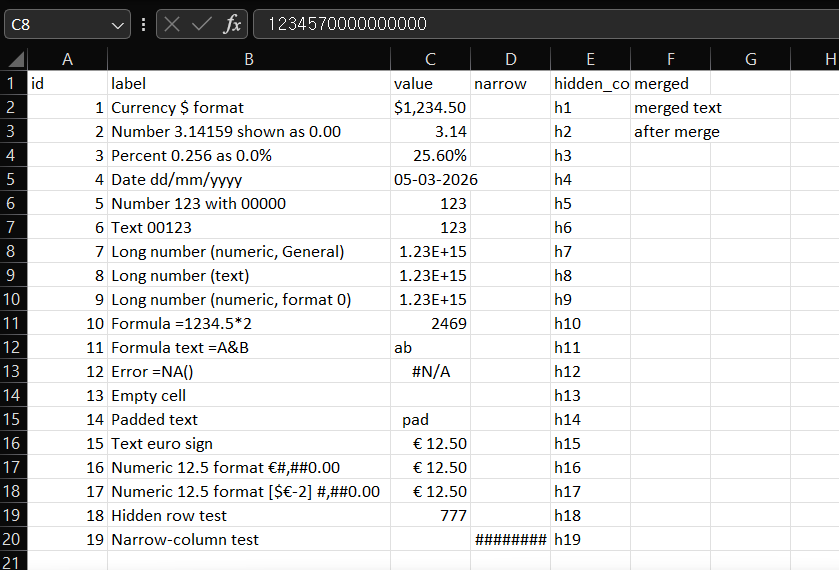
    Excel sheet after reopening the saved CSV, with cell C8 showing 1.23E+15 and its formula bar showing 1234570000000000, and the 00123 cells shown as 123
    The saved CSV reopened with File > Open: C8 now holds 1234570000000000, and 00123 became 123.
    • 00123 came back as 123 in both C6 and C7, including the cell that was text in the source.
    • The General-format long number, saved as 1.23457E+15, came back with 1234570000000000 in the formula bar, and the number format box showed Scientific.
    • The text cell saved as 1234567890123456 came back as a number, with 1234567890123450 in the formula bar.
    • The dollar amount, the percent and the date appeared as the file had them: $1,234.50, 25.60% and 05-03-2026.

    So the digits and zeros that were not in the file could not come back, and the ones that were in the file were read as numbers. We closed the workbook without saving. We did not reopen the UTF-8 file this way.

    Hidden Rows, Hidden Columns, Merged Cells and Narrow Columns

    We kept this part short. All of it comes from the same two files.

    • Hidden row: a row we hid (Hidden row test, value 777) was in the file.
    • Hidden column: a column we hid (cells h1 to h19) was in the file.
    • Merged cells: we merged F2 and G2. The file has merged text in the F2 position and an empty field for G2. Every line in the file ended with a comma, which adds an empty last field. We did not test what causes the trailing comma.
    • Narrow column: a number in a column too narrow to show it displayed ## in Excel, but the file had the formatted value "1,234,567.89", not ##.

    Euro Amounts and a Space in the Price

    We put the same amount, 12.5, in cells with two number formats, plus one text cell with €12.50:

    CellFormatSaved as
    Text €12.50text€12.50
    12.5€#,##0.00€12.50
    12.5[$€-2] #,##0.00€ 12.50 (with a space)

    The space in the last row comes from a space we typed into that format code. We did not test the cells from our earlier encoding post, so this does not explain them.

    The euro sign itself differed between the two files. In the UTF-8 file it was the three bytes E2 82 AC. In the “CSV (Comma delimited)” file it was the single byte 80, not a question mark. Microsoft’s page for these formats says the euro symbol is converted to a question mark in the comma-delimited format. We do not know why our file differs from that description, and we did not look for the cause. The page lists Excel for Microsoft 365, 2024 and 2021 as applying.

    How We Would Use This

    • Before saving a CSV, look at what the cells display. In our test, that is what the file held, formats and all.
    • Keep long IDs as text, as in C9, if every digit must reach the file.
    • Check that Show Formulas is off before you save.
    • Keep the original workbook, and save the CSV under a new file name.

    Things to Know

    • Scope. Everything above comes from one test sheet on Excel 2021 (Version 2608) with Korean regional settings and a comma list separator. Other formats, other Excel versions and Mac may behave differently.
    • Not tested. Show Formulas with “CSV (Comma delimited)”, reopening the UTF-8 files, other date and currency formats, text cells with other kinds of spaces, very long text, other programs reading these files, a different list separator, and Excel for the web.
    • Unconfirmed. Why the General cell held 1234567890123460 after the file was opened, why the euro sign was 80 instead of a question mark, and what causes the trailing comma in each line.

    One-line Summary

    In our Excel 2021 test, a CSV held the values as the cells displayed them, including scientific notation for a long General-format number, while Show Formulas wrote formulas and raw values instead, and reopening the file could not bring back digits or leading zeros that were not in it.

    Sources

    Screenshots and behavior described as “we saw” come from our own test in Excel 2021 on one setup. Microsoft documentation used for the points noted above:

    • Excel formatting and features that are not transferred to other file formats: for CSV (Comma delimited), it says the format saves the text and values as displayed, and that a formula shown instead of its result is saved as text. It also mentions the euro symbol being converted to a question mark. As we read it, the page does not address numbers longer than 15 digits, hidden rows or columns, or merged cells, so those results come from our test.
  • Excel Save as CSV: How Commas, Quotes and Line Breaks Are Written

    When a cell holds a comma, a double quote, or a line break, a CSV file needs some way to keep that cell in one piece. We saved a small test sheet as a CSV in Excel, read the bytes of the files, and reopened them to see what Excel wrote and what came back.

    This guide shows the sheet we used, the exact text Excel saved for each kind of cell, and what we saw when we opened those files again.

    Tested in: Excel 2021 desktop (Version 2608) with an English interface, on Windows with Korean regional settings (list separator ,, decimal point .). Everything below describes what happened on that one setup. We did not test other Excel versions, other regional settings, or Mac, and results may differ there.

    Our Test Sheet

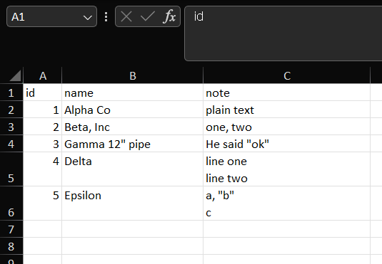
    We created a workbook with a script rather than typing it in Excel, with five data rows. Each row has a different kind of cell content:

    idnamenoteWhat it tests
    1Alpha Coplain textNo special characters
    2Beta, Incone, twoCommas
    3Gamma 12″ pipeHe said “ok”Double quotes
    4Deltaline one (line break) line twoA line break inside a cell
    5Epsilona, “b” (line break) cA comma, quotes and a line break together
    Excel test sheet with columns id, name and note: row 2 has Beta, Inc and one, two, row 3 has Gamma 12" pipe and He said "ok", and rows 4 and 5 have two-line cells
    The test sheet: commas, double quotes, and line breaks inside cells.

    The line breaks are real breaks inside the cell, so the cell shows two lines. We kept this workbook as it was and saved new files from it.

    Saving the Sheet as CSV

    We used File > Save As and saved the sheet twice under new file names, once as “CSV UTF-8 (Comma delimited)” and once as “CSV (Comma delimited)”. Excel did not show a warning dialog for either save. If you are choosing between the two formats, our byte-level comparison of both save options covers the BOM and special-character differences. Here we only look at how the cells were written.

    What Excel Wrote

    We looked at the bytes of both files outside Excel. This is the text of the UTF-8 file, without its invisible BOM at the start:

    id,name,note
    1,Alpha Co,plain text
    2,"Beta, Inc","one, two"
    3,"Gamma 12"" pipe","He said ""ok"""
    4,Delta,"line one
    line two"
    5,Epsilon,"a, ""b""
    c"
    • A cell with plain text and no special characters was written as it is, without quotes: Alpha Co and plain text. The header row and the numbers were also written without quotes.
    • A cell with a comma was wrapped in double quotes: "Beta, Inc" and "one, two".
    • A cell with a double quote was wrapped in double quotes, and each double quote inside the cell was written twice: He said "ok" became "He said ""ok""", and Gamma 12" pipe became "Gamma 12"" pipe".
    • A cell with a line break was wrapped in double quotes, and the break stayed inside them, so the text of one row takes two lines in the file.
    • Each row ended with a carriage return and a line feed (bytes 0D 0A), including the last row. The line break inside a cell was a single line feed (0A).
    • The file saved as “CSV (Comma delimited)” had the same bytes as the UTF-8 file, except that it did not have the three-byte BOM at the start. The UTF-8 file was 157 bytes and the other was 154 bytes. Our test text uses only plain ASCII characters, so this says nothing about accented letters.

    What We Saw When Opening the CSV Again

    We opened the file saved as “CSV (Comma delimited)” with File > Open (Ctrl+O). It opened without the Text Import Wizard, with the header and all five data rows, one cell per field. We did not reopen the UTF-8 file this way.

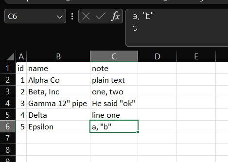
    Excel sheet after reopening the saved CSV with the same five rows, and the formula bar for cell C6 showing a, "b" followed by c on a second line
    The saved CSV reopened with File > Open; the formula bar for C6 shows two lines.

    The Beta, Inc and one, two cells stayed in one cell each, and the quotes were not shown around the cells. Cell C6 holds the text a, "b" followed by a line break and c; the formula bar shows both lines. The row for Delta shows only its first line, line one, in the grid, which we did not investigate further. We closed the workbook without saving.

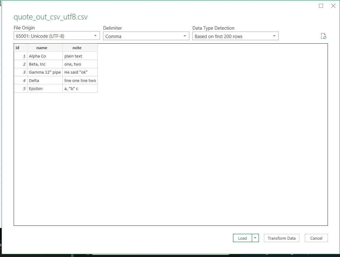
    We also used Data > Get Data > From File > From Text/CSV, this time on the UTF-8 file.

    From Text/CSV preview of the saved UTF-8 CSV with File Origin 65001, Delimiter Comma, and five data rows, with the line breaks in the note column shown as spaces
    The From Text/CSV preview of the UTF-8 file: five rows, with the line breaks shown as spaces.

    Tap the image to view it at full size.

    The preview showed File Origin 65001: Unicode (UTF-8), Delimiter Comma, and five data rows. In the preview, the line breaks in the note column look like spaces (line one line two). We clicked Load, and the Queries & Connections pane said “5 rows loaded”. To check the cells, we typed a formula into a spare cell. LEN of the Delta note was 17, and the ninth character had the code 10, which is a line feed. LEN of the Epsilon note was 8, and its seventh character was also code 10. Gamma 12" pipe and He said "ok" came back with their quotes, one each. So the loaded cells held the line breaks and quotes, even though the preview and the grid did not show the breaks as separate lines.

    How We Would Use This

    • If your cells contain commas, quotes or line breaks, we would let Excel write the CSV rather than edit the file by hand. In our test it quoted every cell that needed it and doubled the quotes inside.
    • Check how the program that reads your CSV treats quoted fields. We only tested Excel, and we did not test any other program.
    • If line breaks inside cells are not wanted in the data, they can be removed before saving; see how to remove line breaks from cells in Excel. We did not test how that affects the saved CSV.
    • Keep the original workbook, and save the CSV under a new file name. A CSV file keeps the text and values, not the sheet formatting.

    For the reverse problem, a CSV that opens in one column, see what happened with a semicolon CSV.

    Things to Know

    • Scope. Everything above comes from one five-row sheet, saved twice on Excel 2021 (Version 2608) with Korean regional settings and a comma list separator. We did not test other Excel versions, other regional settings, or Mac.
    • Not tested. Opening the files in programs other than Excel, double-clicking a CSV in File Explorer, a different list separator, a semicolon-delimited save, cells with leading or trailing spaces, tab characters, a cell with only a double quote, carriage returns inside cells, very long cells, CSV (Macintosh) and CSV (MS-DOS), Unicode Text, files with more than five rows, and Excel for the web.
    • Unconfirmed. We do not know why the grid showed only the first line of the Delta cell after we reopened the file. We also did not check how Excel decides which cells get quotes beyond the cases above.
    • Keep the original. Save under a new file name and keep a copy of the source workbook.

    One-line Summary

    In our Excel 2021 test, saving as CSV wrapped cells with commas, double quotes or line breaks in double quotes, doubled the quotes inside them, kept in-cell line breaks as a single line feed, and the files we reopened came back with one cell per field, the “CSV (Comma delimited)” file through File > Open and the UTF-8 file through From Text/CSV.

    Sources

    Screenshots and behavior described as “we saw” come from our own test in Excel 2021 on one setup. Microsoft documentation used for the points noted above:

  • Excel CSV UTF-8 vs CSV (Comma delimited): What the Saved Files Contained

    Excel’s Save As list has two similar-looking CSV choices: “CSV UTF-8 (Comma delimited)” and “CSV (Comma delimited)”. They do not produce the same file. We saved one small test sheet both ways and looked at the bytes of each result.

    This guide shows what we saw in the Save As dialog, how the two files differed at the start and in the accented letters, and which characters did not survive in one of them.

    Tested in: Excel 2021 desktop (Version 2608) with an English interface, on Windows with Korean regional settings (list separator ,, decimal point .). Everything below describes what happened on that one setup. We did not test other Excel versions, other regional settings, or Mac, and results may differ there.

    Our Test Data

    The source was a five-row CSV file that we created ourselves. It is UTF-8 with a byte order mark (BOM), 201 bytes:

    id,name,city,price
    1,José Álvarez,São Paulo,€12.50
    2,Zoë Müller,Zürich,€8.00
    3,Chloé Dupont,Montréal,€15.25
    4,Søren Ødegård,København,€9.90
    5,Łukasz Nowak,Łódź,€7.00

    Row 5 is there on purpose. The letters Ł and ź are not in the Windows-1252 character set, so they show whether a save loses characters. We did not test Korean, Japanese, Chinese, or other scripts.

    We opened the file directly with File > Open (Ctrl+O). As in our earlier encoding test, the Text Import Wizard appeared first with File origin 65001 : Unicode (UTF-8). We ticked Comma, clicked Finish, and the sheet showed the names and the euro sign correctly. The prices appeared as € 12.50 with a space. We did not check why.

    The Two Save As Choices

    We did not save over the source file. We used File > Save As (F12) in the same folder and typed a new file name each time.

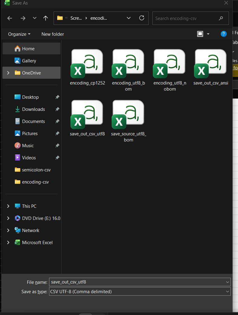
    Excel Save As dialog with the file name save_out_csv_utf8 and Save as type set to CSV UTF-8 (Comma delimited)
    The Save As dialog with “CSV UTF-8 (Comma delimited)” shown in “Save as type”.

    When the Save As dialog opened on this workbook, the “Save as type” box already showed “CSV UTF-8 (Comma delimited)”. We saved this one as save_out_csv_utf8.csv.

    Excel Save As dialog with the file name save_out_csv_ansi and Save as type set to CSV (Comma delimited)
    The same dialog with “Save as type” changed to “CSV (Comma delimited)”.

    For the second file, we changed “Save as type” to “CSV (Comma delimited)” and saved it as save_out_csv_ansi.csv. We chose the name “ansi” ourselves; Excel does not label the format that way.

    Excel did not show a warning dialog when we saved either file. A yellow “POSSIBLE DATA LOSS” banner was already on the sheet when we opened the source CSV and stayed there; it is not in the screenshots.

    What Was Inside Each File

    We looked at the bytes of both files outside Excel, with a small script that prints the hex values and tries decoding the text.

    On a phone-width screen, the comparison table below was wider than the page in our preview, so swipe it left and right to see every column.

    Source fileCSV UTF-8 (Comma delimited)CSV (Comma delimited)
    File size201 bytes206 bytes177 bytes
    Starts with EF BB BF (BOM)YesYesNo
    Line endingsCRLFCRLFCRLF
    é as bytesC3 A9C3 A9E9
    € as bytesE2 82 ACE2 82 AC80
    Ł and źKept (UTF-8)Kept (UTF-8)Both became 3F (?)
    Strict UTF-8 decode in our scriptSucceededSucceededFailed (byte E9)
    Strict Windows-1252 decode in our scriptFailed (byte 81)Failed (byte 81)Succeeded
    Original text when read as Windows-1252Not checkedNot checkedCorrect except row 5

    The decode rows describe what our script could do with each file’s bytes. A failed strict decode only means that the script could not map every byte to a character. We did not check how Excel or any other program shows the two UTF-8 files when they are read as Windows-1252, so we do not draw a conclusion about that.

    • The UTF-8 save kept the BOM, and every letter in our five rows came back unchanged when decoded as UTF-8.
    • The “CSV (Comma delimited)” save had no BOM and stored accented letters such as é and the euro sign as single bytes. Decoded as Windows-1252, the text reads correctly, apart from row 5.
    • Row 5 lost three characters in that file: Łukasz became ?ukasz and Łódź became ?ód?. The other accented letters in our data were stored as single bytes. We counted three ? bytes in the whole file.
    • In both saved files the prices were written as € 12.50, with a space, instead of the €12.50 in the source. Both files did this, so we do not tie it to the encoding. We did not check the cell format.
    • The ANSI file did not decode as Korean (code page 949) in our check. We did not look at the Windows system code page setting itself, so we only say what the bytes show: they decode as Windows-1252.

    What Excel Showed When We Reopened the Windows-1252 File

    We opened save_out_csv_ansi.csv directly with File > Open. It opened without the Text Import Wizard.

    Excel sheet after reopening save_out_csv_ansi.csv, where row 5 shows ?ukasz Nowak and ?ód? and the other rows look correct
    The “CSV (Comma delimited)” file reopened: row 5 reads ?ukasz Nowak and ?ód?.

    Row 5 reads ?ukasz Nowak and ?ód?. In the bytes of this saved file, the positions of Ł and ź hold 3F (?), as the table above shows. From this saved CSV alone we cannot recover the original letters. The other four rows looked correct on our screen. We closed the workbook without saving.

    We did not reopen the UTF-8 save, and we did not open either saved file with Data > From Text/CSV. We therefore do not say how Excel shows the UTF-8 save when reopened.

    How We Would Choose

    • If your data has characters outside Western European languages, such as Ł and ź in our test, we would use “CSV UTF-8 (Comma delimited)” on this setup. In our test, only that file kept all of them.
    • If the receiving program needs a particular encoding, check what it expects before saving. We did not test any receiving program.
    • Keep the original workbook. A CSV file stores values only, so we would save the sheet as an .xlsx too if you need the formatting.
    • After saving, check the result outside Excel if the characters matter. If a letter from the original appears as ? in the saved file, as Ł and ź did in ours, the saved CSV alone cannot give the original letter back; go back to the original workbook or source data. A ? can also be a real question mark in the data, so compare with the original before concluding anything.

    If you later open a CSV and see broken accents, see garbled CSV characters in Excel. Our saved files used a comma as the separator, which matches the list separator on our Windows setup. We did not change that setting; if a CSV opens in one column, see what happened with a semicolon CSV.

    Things to Know

    • Scope. Everything above comes from one five-row file, saved twice on Excel 2021 (Version 2608) with Korean regional settings. We did not test other Excel versions, other regional settings, or Mac.
    • Not tested. Korean and other non-Latin scripts, UTF-16 or “Unicode Text”, the “CSV (Macintosh)” and “CSV (MS-DOS)” choices, changing the Windows list separator, reopening the UTF-8 save, opening either saved file with From Text/CSV, receiving programs, files with more than five rows, and Excel for the web.
    • Unconfirmed. We do not know why the source file with a BOM opened in the Text Import Wizard, why the price text gained a space on saving, or whether the same two choices behave this way on other setups.
    • Keep the original. Save under a new file name and keep a copy of the source CSV.

    One-line Summary

    In our Excel 2021 test, “CSV UTF-8 (Comma delimited)” produced a file with a BOM that kept every letter in our data, while “CSV (Comma delimited)” produced a file without a BOM that our script could decode as Windows-1252 and turned Ł and ź into question marks.

    Sources

    Screenshots and behavior described as “we saw” come from our own test in Excel 2021 on one setup. We did not rely on Microsoft documentation for the results above.
  • Garbled CSV Characters in Excel: Check the Encoding

    A CSV with names like José or Zürich can open in Excel as José or Zürich, and a euro sign can turn into €. One possible cause is an encoding mismatch: the program reading the file uses a different character set than the one used to save it. In our test we could not see which encoding Excel used when it opened a file directly, so we describe only what the screen showed.

    This guide shows what happened when we opened the same four-row test data saved three ways, and how Data > From Text/CSV let us see and change the File Origin before loading anything.

    Tested in: Excel 2021 desktop (Version 2608) with an English interface, on Windows with Korean regional settings. Everything below describes what happened on that one setup. We did not test other Excel versions, other regional settings, or Mac, and results may differ there.

    Our Test Files

    We saved the same four rows as three CSV files, so we know exactly how each one is encoded:

    id,name,city,price
    1,José Álvarez,São Paulo,€12.50
    2,Zoë Müller,Zürich,€8.00
    3,Chloé Dupont,Montréal,€15.25
    4,Søren Ødegård,København,€9.90
    • UTF-8 without a byte order mark (BOM)
    • UTF-8 with a BOM
    • Windows-1252, the Western European Windows code page

    The data uses accented letters and a euro sign instead of non-Latin text. We did not test Korean, Japanese, Chinese, or other scripts.

    Opening the UTF-8 File Without a BOM Directly

    We opened the UTF-8 file without a BOM directly with File > Open (Ctrl+O), not through the Data tab. We did not test double-clicking the file in File Explorer.

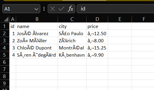
    Excel sheet after opening the UTF-8 CSV without a BOM directly: the header id, name, city, price is normal, but names and prices are garbled, such as José Ãlvarez, São Paulo and €12.50, where the second character looks like a comma
    Opened directly: the header is fine, but the names, cities and prices are garbled. The yellow banner that appeared on our screen is not in the screenshot.
    • The header id,name,city,price looks normal. The names, cities, and prices do not: José Ãlvarez, São Paulo, Zürich, €12.50 (the second character of the garbled euro sign looks like a comma on screen; when we checked the cell with Excel’s UNICODE function it was code 8218, a low single quotation mark, which we write as ‚).
    • The garbled prices sit on the left side of their cells, like text.
    • On our screen, a yellow “POSSIBLE DATA LOSS” banner also appeared. It is not in the screenshot.

    We did not save this workbook. The banner talks about saving in the .csv format, so we closed the file without saving over the original.

    Opening the UTF-8 File With a BOM Directly

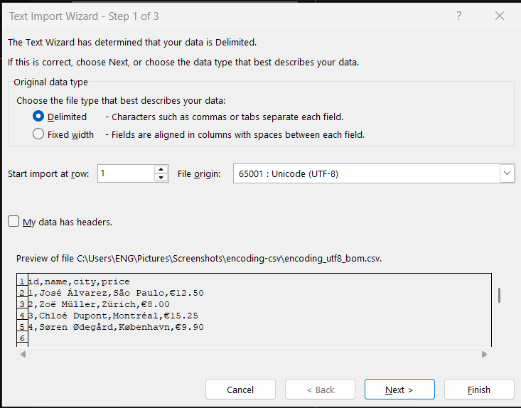
    We used the same File > Open steps on the UTF-8 file that has a BOM. This time Excel did not open the file straight into the sheet. The Text Import Wizard appeared first, with File origin set to 65001 : Unicode (UTF-8) and a preview that shows the accents and the euro sign correctly.

    Text Import Wizard step 1 of 3 with Delimited selected, File origin 65001 : Unicode (UTF-8), and a preview showing José Álvarez, São Paulo and €12.50 correctly
    The UTF-8 file with a BOM opened in the Text Import Wizard first. File origin shows 65001, and the preview looks right.

    We saw the wizard each of the four times we opened this file, including twice after restarting Excel. We do not know why it appeared here and not for the other files, and we did not test whether the Excel setting for legacy import wizards plays a role.

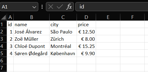
    In the wizard, step 2 showed Semicolon ticked, so we ticked Comma instead and clicked Finish. On our screen the sheet then showed José Álvarez, São Paulo, Zürich and € 12.50 correctly. That sheet is not in a screenshot.

    Microsoft’s page on opening UTF-8 CSV files says a UTF-8 file saved with a BOM opens normally and that, for a file without one, you can use From Text/CSV or the Text Import Wizard (see the sources). We saw a wizard for the BOM file, so we would not describe our result as “it simply opens”. We did not test whether a file with a BOM opens straight into a sheet on other setups.

    Opening the Windows-1252 File Directly

    The Windows-1252 file opened straight into the sheet, with no wizard.

    Excel sheet after opening the Windows-1252 CSV directly with names José Álvarez, Zoë Müller, Chloé Dupont and Søren Ødegård and prices such as € 12.50 shown correctly
    The Windows-1252 file opened straight into the sheet, with the accents and euro sign intact.

    The names, cities, and prices look right: José Álvarez, Zoë Müller, København. The prices appear right-aligned with a euro sign, such as € 12.50. We do not know whether Excel read the file with the Windows-1252 code page or detected it some other way, and we did not look at which settings are involved. We did not open this file with Data > From Text/CSV, so we did not try 1252 on it.

    So on our setup, the same four rows came out garbled from the UTF-8 file without a BOM and correct from the other two files (the BOM file after the wizard).

    Check the File Origin With Data > From Text/CSV

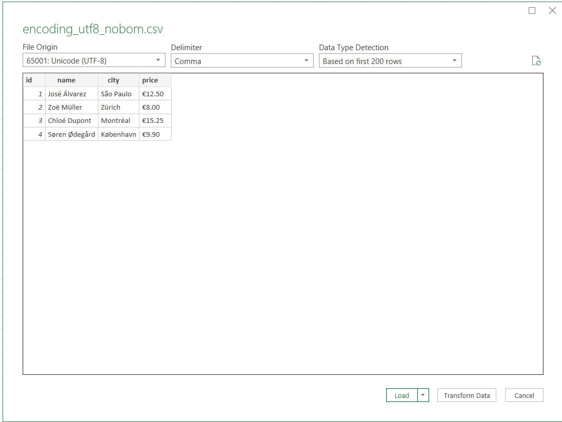
    In a blank workbook we used Data > Get Data > From File > From Text/CSV and chose the UTF-8 file without a BOM. Excel showed a preview window before loading anything.

    From Text/CSV preview of the UTF-8 file without a BOM with File Origin 65001: Unicode (UTF-8), Delimiter Comma, and names such as José Álvarez and Søren Ødegård shown correctly
    From Text/CSV preview of the same file that was garbled when opened directly: File Origin shows 65001 and the accents look right.

    Tap the image to view it at full size.

    The window showed File Origin 65001: Unicode (UTF-8), Delimiter Comma, and Data Type Detection Based on first 200 rows. We did not change any of them. The preview shows José Álvarez, Zoë Müller, and Søren Ødegård correctly, and the prices appear on the left side as €12.50.

    We do not know how Excel chose 65001 here. For this file, the same one that came out garbled when opened directly, the preview was correct without any change from us.

    We clicked Load. On our screen the table showed the names, cities, and prices correctly, and the Queries & Connections pane said “4 rows loaded”. We did not take a screenshot of the loaded table, and we did not test refreshing the query.

    What the Wrong File Origin Looks Like

    To see what a wrong choice looks like, we opened the same preview of the UTF-8 file and changed only File Origin to 1252: Western European (Windows). We know this file is UTF-8, so 1252 is the wrong value for it.

    From Text/CSV preview with File Origin changed to 1252: Western European (Windows), which does not match this UTF-8 file, showing garbled names such as José Ãlvarez and prices such as €12.50
    Only File Origin changed, to 1252, which does not match this UTF-8 file: the preview is garbled. This was a deliberate wrong choice.

    Tap the image to view it at full size.

    The preview now showed José Ãlvarez, São Paulo, Zürich and €12.50. These look like the garbled text from opening the file directly. That was a deliberate wrong choice for this test. We loaded it once into a scratch workbook only to check the characters, and closed that workbook without saving. The characters were the same as in the directly opened sheet: â, then ‚ (code 8218), then ¬. We did not check the preview itself character by character, and we did not check which code page Excel used when the file opened directly, so we can only say the screens look alike.

    Microsoft’s Text Import Wizard page describes File origin as the character set used in the text file, says you can usually leave it at the default, and says to change it when the file was made with a different character set (see the sources).

    A Check You Can Do on Your Own File

    • Find out how the file was saved. Look at the export settings where the file was created, or ask whoever supplied it. We did not test any other way of finding out, such as looking at the file in a text editor.
    • Open the file with Data > Get Data > From File > From Text/CSV, not with a double click or File > Open, and look at the preview before you load anything.
    • Pick the File Origin that matches the encoding you were told. 65001 fit our UTF-8 test files, but it is not the right value for every CSV. A file saved as Windows-1252 would call for 1252, although we did not try that file in From Text/CSV.
    • If you do not know the encoding, ask the file provider. A preview that looks right is a clue, not confirmation, and our test files were ones we created, so we knew their encoding in advance.
    • When the File Origin matches the file and the preview shows the characters you expect, we would click Load. In our test we clicked Load only with 65001 on the UTF-8 file, where the preview was already correct.

    Before you try different settings, keep a copy of the original CSV. If you opened the file directly and made no edits, we would close it with Don’t Save rather than save over the original CSV, then import it again as above. If you do have edits you want to keep, save them under a new file name (for example as an .xlsx) before closing.

    If dates or numbers also come in wrong, see fixing dates after a CSV import and how a decimal comma import behaved in Excel. If the data lands in one column, see what happened with a semicolon CSV.

    Which Way to Open the File

    What you wantWhat we would try first
    Open a CSV whose accents or symbols look garbledClose it with Don’t Save, then Data > From Text/CSV and check the preview
    Choose the File OriginThe one that matches the file’s real encoding (ask the file provider if unsure), then check the preview before Load

    Things to Know

    • Scope. Everything above comes from one four-row test file saved in three ways, on Excel 2021 (Version 2608) with Korean regional settings. We did not test other Excel versions, other regional settings, or Mac.
    • Not tested. Non-Latin scripts such as Korean, other encodings such as UTF-16, double-clicking a CSV in File Explorer, checking the encoding in a text editor, saving a CSV from Excel as CSV UTF-8, opening the Windows-1252 file in From Text/CSV or choosing 1252 for it, the Text Import Wizard File origin list, the Transform Data option, Excel for the web, Power Query code, and files with more than four data rows. Data Type Detection used the first 200 rows in the dialog, and our file had four.
    • Keep the original file. Keep a copy of the source CSV and avoid saving over it. If you have edits to keep, save them under a new name first. If you have no edits and Excel asks whether to save changes when you close, we would choose Don’t Save.
    • Look at the result. After loading, compare a few names and symbols with the original, especially values with accents or a currency sign.

    One-line Summary

    In our Excel 2021 test, a UTF-8 CSV without a BOM opened directly as José and €, the same data opened correctly from the BOM file (through the Text Import Wizard) and from the Windows-1252 file, and Data > From Text/CSV showed a correct preview with 65001, which matched that UTF-8 file, and a garbled one with 1252, which did not.

    Sources

    Screenshots and behavior described as “we saw” come from our own reproduction in Excel 2021 on one setup. Microsoft documentation used for the points noted above:

  • Excel Opens a Semicolon CSV in One Column: How to Split It

    Some exports separate fields with semicolons (;) instead of commas, and the file can still end in .csv. Opened in Excel, such a file may not look like a table at all.

    This guide shows what happened when we opened one small semicolon-separated test file in Excel, why Text to Columns lost part of one row in our test, and how Data > From Text/CSV kept every value in its own cell.

    Tested in: Excel 2021 desktop (Version 2608) with an English interface, on Windows with Korean regional settings (decimal point ., thousands separator ,, list separator ,). Everything below describes what happened on that one setup. We did not test other Windows regional settings, other Excel versions, or Mac, and results may differ there.

    Our Test File

    The file has a header and four data rows:

    id;name;city;qty;note
    1;Alpha Co;Seoul;12;ok
    2;Beta, Inc;Busan;7;"has; semicolon inside"
    3;Gamma Ltd;Daegu;0;
    4;Delta;Incheon;150;ok

    Two rows are there on purpose. In row 2 of the data, the company name Beta, Inc contains a comma, and the note is written in quotes because it contains a semicolon. In row 3 the last field is empty, so the line ends with ;. What we expected from a correct import is five columns, four data rows, Beta, Inc in one cell, has; semicolon inside in one cell, and an empty note for Gamma Ltd.

    Opening the CSV Directly

    We opened the file directly with File > Open (Ctrl+O), not through the Data tab. We did not test double-clicking the file in File Explorer.

    Semicolon CSV opened directly in Excel: most rows sit in column A as text such as 1;Alpha Co;Seoul;12;ok, while row 3 is split between A3 and B3 at the comma in Beta, Inc
    Opened directly: rows sit in column A with their semicolons, and the Beta, Inc row is split at its comma. The formula bar shows the content of B3.
    • The header and the Alpha Co, Gamma Ltd, and Delta rows each sit entirely in column A, semicolons and all.
    • The Beta, Inc row is split in two, but at the comma, not at a semicolon. A3 shows 2;Beta, and the formula bar for the selected cell B3 shows Inc;Busan;7;"has; semicolon inside".
    • On our screen, the title bar also said Read-Only and a yellow “POSSIBLE DATA LOSS” banner appeared. Neither is in the screenshot.

    Our reading is that Excel split only where it found a comma, and the list separator on our Windows setup is a comma. We did not change that setting, so we cannot say it is the cause. Microsoft’s page on importing text files does not explain how Excel picks the delimiter when you open a .csv directly (see the sources).

    Method 1: Data > From Text/CSV

    In a blank workbook we used Data > Get Data > From File > From Text/CSV and chose the file. Excel showed a preview window before loading anything.

    From Text/CSV preview with Delimiter set to Semicolon and a five-column preview where Beta, Inc and has; semicolon inside each sit in one cell
    From Text/CSV preview: Delimiter shows Semicolon, Beta, Inc is one cell, has; semicolon inside is one cell, and the note for Gamma Ltd is empty.

    Tap the image to view it at full size.

    The window showed three settings: File Origin 949: Korean, Delimiter Semicolon, and Data Type Detection Based on first 200 rows. We did not change any of them. The preview had five columns. Beta, Inc sat in one cell, has; semicolon inside sat in one cell, the note for Gamma Ltd was empty, and the id and qty values were right-aligned.

    We do not know how Excel chose Semicolon here. Microsoft’s page says that with From Text/CSV you can pick a delimiter and preview the result before importing, so the choice is yours to check. Our file contains only plain ASCII characters, and we did not test other encodings.

    We clicked Load.

    Worksheet table after Load with columns id, name, city, qty and note and four data rows, Beta, Inc in one cell, has; semicolon inside in one cell, and an empty note for Gamma Ltd
    After Load: four data rows in five columns. Beta, Inc and has; semicolon inside each stay in one cell, and the Gamma Ltd note stays empty.

    The table filled A1:E5. Excel’s Queries & Connections pane said “4 rows loaded”, which is not in the screenshot. We compared the cells with the file text by eye: Beta, Inc and has; semicolon inside stayed in single cells, and the empty note for Gamma Ltd stayed empty, matching the trailing ; in the file. We did not run formulas such as ISNUMBER on the loaded columns, and we did not test refreshing the query or moving the file.

    Method 2: Text to Columns

    If the file is already open in one column, Text to Columns on column A can split it. We selected column A (the selection is not visible in the screenshots) and used Data > Text to Columns > Delimited > Next. In step 2, only Semicolon was ticked, and the text qualifier was a double quote.

    Text to Columns wizard step 2 with only Semicolon ticked and a data preview of five columns in which the Beta row stops after Beta
    Text to Columns, step 2: only Semicolon is ticked. The preview shows what is in column A, so the Beta, Inc row stops after “Beta”.

    The data preview shows only what is in column A, so the Beta, Inc row stops after Beta. When we clicked Finish, Excel asked whether to replace existing data.

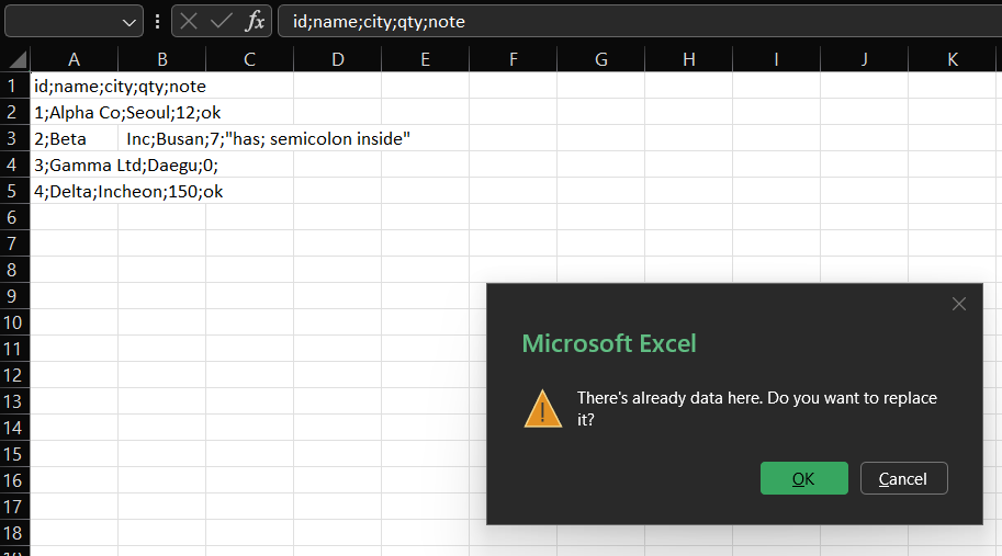
    Excel dialog reading There's already data here. Do you want to replace it? with OK and Cancel buttons, shown over the one-column semicolon data
    The warning Excel showed when we clicked Finish.

    That fits what we saw earlier: B3 already held the piece after the comma, and the split would write into column B. We clicked OK.

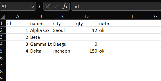
    Worksheet after Text to Columns with id, name, city, qty and note in columns A to E; row 3 shows only 2 and Beta, with empty city, qty and note cells
    After OK: the other rows split into five columns, but row 3 keeps only 2 and Beta. The Gamma Ltd name looks cut off because the column is narrow.

    Rows for Alpha Co, Gamma Ltd, and Delta split into five columns. The Beta, Inc row did not: it ended up with only 2 and Beta, and the city, qty, and note cells are empty. The text after the comma, Inc;Busan;7;"has; semicolon inside", is no longer on the sheet. We would treat that as lost data. That is what happened in this test; we did not test other files, so we cannot say every semicolon file behaves this way.

    What we would do: before running Text to Columns on a directly opened file, check whether any cell to the right of column A already has data, as our row 3 did. We did not test other ways around this, such as clearing column B first or changing the Destination box. If the split has already damaged the sheet, we would not try to repair it. We would close the workbook with Don’t Save so the original file is never overwritten, and import the original again with Data > From Text/CSV (Method 1). In our test we never saved the workbook, and Method 1 afterwards loaded the same file with all four data rows intact.

    Which Method to Use

    SituationMethod we would try first
    You have the CSV file and want every value in its own cellData > From Text/CSV
    The file is already open in one columnText to Columns, after checking for data to the right of column A

    On our test file, From Text/CSV kept all four data rows intact, and Text to Columns lost part of one row. If numbers or dates come in wrong after an import, see how a decimal comma import behaved in Excel and fixing dates after a CSV import.

    Things to Know

    • Scope. Everything above comes from one five-line test file on Excel 2021 (Version 2608) with Korean regional settings and a comma list separator. We did not test other Windows regional settings, other Excel versions, or Mac.
    • Not tested. We did not change the Windows list separator. Microsoft’s page describes it, under Region settings > Additional settings > Numbers, as the default separator for new text files saved as .csv and says the change affects all programs. We did not test whether it changes how a directly opened file is split. We also did not test renaming the file to .txt to get the Text Import Wizard, the Transform Data option, other delimiters, other encodings such as UTF-8 with a byte order mark, quoted fields that contain line breaks, Excel for the web, or files with more than four data rows. Data Type Detection used the first 200 rows in the dialog, and our file had four.
    • Keep the original file. Do not save over the source CSV. If Excel asks whether to save changes to it when you close it, we would choose Don’t Save. If a split has gone wrong, re-import the original with Data > From Text/CSV.
    • Look for lost cells. After any split, compare the row count and a few rows with the original text, especially rows with commas, quotes, or empty last fields.

    One-line Summary

    In our Excel 2021 test, a semicolon CSV opened directly landed mostly in column A, Text to Columns on column A lost part of the Beta, Inc row, and Data > From Text/CSV kept every value in its own cell.

    Sources

    Screenshots and behavior described as “we saw” come from our own reproduction in Excel 2021 on one setup. Microsoft documentation used for the points noted above:

  • How to Import Numbers With a Decimal Comma (1.234,56) in Excel

    Some exports write the number one thousand two hundred thirty-four and fifty-six hundredths as 1.234,56: a dot between the thousands and a comma before the decimals. Others write 1,234.56. Both are meant to be the same number, but Excel does not necessarily read them the same way.

    This guide shows what we observed when we opened one small test CSV containing both styles, and three ways to turn the comma-decimal column into real numbers. The one we would use for files you import repeatedly is setting a locale in Power Query.

    Tested in: Excel 2021 desktop (Version 2608) with an English interface, on Windows with Korean regional settings (decimal point ., thousands separator ,). Everything below describes what happened on that one setup. We did not test other Windows regional settings, other Excel versions, or Mac, and results may differ there.

    Our Test File

    The CSV has six rows and two amount columns. In each row, the two columns are meant to be the same number, written in two styles:

    ColumnExample (first row)Style
    amt_us_style"1,234.56"comma for thousands, dot for decimals
    amt_eu_style"1.234,56"dot for thousands, comma for decimals

    The six intended values are 1234.56, 0.5, 1234567.89, 12, 999.99, and 1234, and they add up to 1,238,048.94. Because the values contain commas, they are written in quotes in the file.

    Row 6 is the one to watch. Its comma-decimal value is 1.234. In this file we mean that as one thousand two hundred thirty-four, with the dot as a thousands separator. A reader who sees 1.234 on its own could also read it as one point two three four, so the intended value is something we decided for the test file, not something Excel can know. We chose 1234 as the intended value for this file; the text 1.234 alone cannot tell you which one the file’s author meant. Check the source system or ask the file’s author to confirm what the value means.

    Opening the CSV Directly

    We opened the file directly in Excel, not through the Data tab, and added a few helper columns (E to H) to check each cell.

    CSV opened in Excel: the amt_us_style column holds right-aligned numbers, the amt_eu_style column holds left-aligned text such as 1.234,56, and only row 6 shows 1.234 as a number
    Opened directly: the comma-decimal text stays text, except row 6 (1.234), which became a number. Columns E to H are helper cells we added; (text) is what our helper prints for a non-number.

    Tap the image to view it at full size.

    • The amt_us_style column came in as numbers. ISNUMBER returned TRUE in all six rows and our helper showed 1234.56, 0.5, 1234567.89, 12, 999.99, and 1234.
    • In amt_eu_style, rows 1 to 5 (1.234,56, 0,50, 1.234.567,89, 12,00, 999,99) stayed left-aligned text, and ISNUMBER returned FALSE.
    • Row 6, 1.234, was different. Excel turned it into a number, and our helper shows it as 1.2340. That is not the 1234 we intended, and there was no error or warning. This is the kind of silent mistake to look for.

    We also tried =VALUE() on the text cells in rows 1 to 5, and it returned #VALUE!. We did not capture that in an image.

    If Excel Has Already Turned a Value Into a Number

    Row 6 shows the risk. Once Excel has read 1.234 as the number 1.234, the cell no longer holds the original text, so the file’s intent is no longer visible in the cell. Changing the cell’s number format only changes how the stored value is displayed, and we did not test changing Windows regional settings after the fact. Neither tells Excel what the file’s author meant.

    What we would do instead is keep the original CSV unchanged and import it again from there. Work on a copy, and if Excel asks whether to save changes to the CSV when you close it, we would choose Don’t Save so the original text stays as it was. Then re-import the original with a locale that matches how its numbers are written (Method 1 below), and check a few values you can verify, such as a total.

    Importing With Data > From Text/CSV

    Next we imported the same file with Data > From Text/CSV and opened Transform Data. Power Query had already added a type-conversion step on its own.

    Power Query Editor formula bar setting amt_us_style to type number and amt_eu_style to type text, with the comma-decimal column showing 1.234,56 and 1.234 as text
    Power Query’s automatic step: amt_us_style becomes type number, amt_eu_style stays type text.

    Tap the image to view it at full size.

    The formula bar shows amt_us_style set to type number and amt_eu_style set to type text. Row 6 stayed text here (1.234) instead of becoming 1.234 as it did when we opened the file directly. We also saw the step listed in the Applied Steps pane (Source, Promoted Headers, Changed Type), which is not part of the screenshot.

    So the comma-decimal column is still text at this point, and the next step is to tell Power Query how those numbers are written.

    Method 1: Change Type With Locale in Power Query

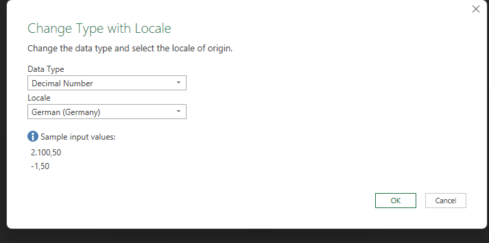
    In the editor we right-clicked the amt_eu_style column header and chose Change Type > Using Locale. In the dialog we set Data Type to Decimal Number and Locale to German (Germany).

    Change Type with Locale dialog with Data Type set to Decimal Number, Locale set to German (Germany), and sample input values 2.100,50 and -1,50
    Change Type with Locale: Decimal Number and German (Germany). The sample input values show the format this locale expects.

    We picked German (Germany) because the dialog’s sample input values (2.100,50 and -1,50) show the dot-thousands, comma-decimal style our column uses. We did not try other locales.

    After OK, the editor added a Changed Type with Locale step, and both amount columns showed the intended numbers:

    Power Query Editor with a formula bar reading Table.TransformColumnTypes with type number and de-DE, and the amt_eu_style column showing 1234.56, 0.5, 1234567.89, 12, 999.99 and 1234
    After Using Locale: the formula bar ends with "de-DE", and amt_eu_style shows the same six values as amt_us_style.

    Tap the image to view it at full size.

    The formula bar reads:

    = Table.TransformColumnTypes(#"Changed Type", {{"amt_eu_style", type number}}, "de-DE")

    The third argument, "de-DE", is the locale. Row 6 now reads 1234, which matches what we intended for the file.

    Then we used Close & Load and added check columns next to the loaded table.

    Loaded worksheet table with both amount columns showing the same values, with ISNUMBER TRUE in both check columns and a sum of 1238048.94
    Loaded to the sheet: both columns are numbers, and the sum matches the 1,238,048.94 we expected. Columns E to G and the sum cell are helper cells we added.

    In the loaded sheet, ISNUMBER returned TRUE for both columns, and the six values were 1234.56, 0.5, 1234567.89, 12, 999.99, and 1234 in both. The sum of the converted column was 1238048.94, the total we computed for the intended values. The formula bar in the screenshot shows =ISNUMBER(C2) for the selected check cell.

    What Microsoft’s documentation says about this: the locale you pick in Change Type > Using Locale is applied to that column and takes priority over the Power Query locale setting and over the operating system’s settings (see the first source below). The documentation’s own example is about dates, and it does not mention number separators, so what we show here for numbers comes from our test, not from that page.

    Method 2: Text to Columns With Decimal and Thousands Separators

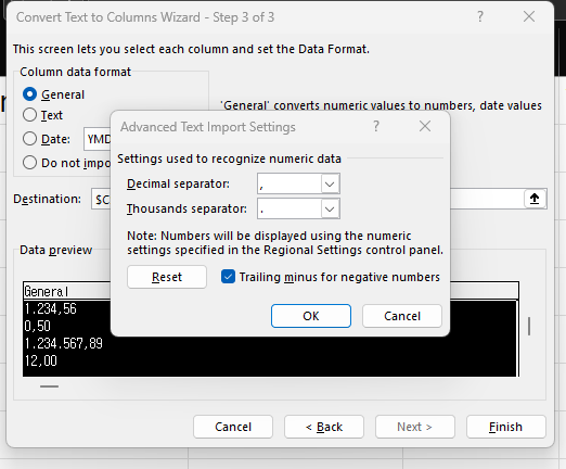
    If the text is already in cells and you do not want to use Power Query, Text to Columns can convert it in place. We selected the comma-decimal text cells (C2:C7 in a working copy) and used Data > Text to Columns > Delimited > Next (with only Tab ticked as the delimiter) > Next. In step 3 we clicked Advanced and entered a comma as the decimal separator and a dot as the thousands separator.

    Advanced Text Import Settings dialog with the decimal separator set to a comma and the thousands separator set to a dot
    Text to Columns, step 3 > Advanced: decimal separator "," and thousands separator ".".

    In that dialog, the “Trailing minus for negative numbers” box was ticked when we got to it; we did not change it. After OK and Finish, the cells became numbers:

    Worksheet after Text to Columns: the amt_eu_style column now shows right-aligned numbers matching amt_us_style, and both ISNUMBER check columns return TRUE
    After Text to Columns: amt_eu_style matches amt_us_style, and ISNUMBER is TRUE for both. Columns E to H are helper cells we added.

    Tap the image to view it at full size.

    The six values were 1234.56, 0.5, 1234567.89, 12, 999.99, and 1234, the same as the intended values. The cells now display with thousands commas (for example 1,234,567.89); we did not check which number format Excel applied. Row 6 had already become the number 1.234 when we opened the file directly. Text to Columns still gave 1234 for it, because we told it the dot is a thousands separator, but Excel itself had read it as 1.234 before that. Text to Columns overwrites the original cells, so keep a copy of the column first.

    Method 3: NUMBERVALUE on Text Cells

    NUMBERVALUE converts text to a number and lets you say which characters are the decimal and thousands separators. Microsoft describes it as converting text to a number “in a locale-independent way” (see the sources). We tried it on a column that Power Query had loaded as text, that is, without the locale step.

    Worksheet with the comma-decimal text column and a NUMBERVALUE column with the formula bar showing NUMBERVALUE(C4, comma, dot), returning the intended numbers and a sum of 1238048.94
    NUMBERVALUE on the text column: ISNUMBER of the source is FALSE, the results are the intended numbers, and the sum is 1238048.94. Columns E and F are helper cells we added.

    The formula bar shows =NUMBERVALUE(C4,",",".") for the selected cell. The second argument is the decimal separator (a comma) and the third is the group separator (a dot). In this test the formula returned 1234.56, 0.5, 1234567.89, 12, 999.99, and 1234, and their sum was 1238048.94. ISNUMBER of the source column was FALSE, so the formulas were converting real text. Per Microsoft’s page, NUMBERVALUE is available in Excel 2021, among other versions.

    One thing to watch: in an earlier trial in a working copy, we ran the same NUMBERVALUE(...,",",".") formulas on cells that Text to Columns had already turned into numbers. The results were wrong (1234.56 came out as 123456). We saw this on our setup and did not capture it in an image, but it is a good reason to convert each column once and check ISNUMBER first.

    Which Method to Use

    SituationMethod we would try first
    You import this kind of file repeatedlyPower Query, Change Type Using Locale
    The text is already in the sheet and you want to replace itText to Columns, Advanced separators
    You want to keep the original text beside the resultNUMBERVALUE in a new column

    All three produced the intended six values on our test file on our setup. For other ways to turn text into numbers in bulk, see converting numbers stored as text in Excel. The same locale idea applies to dates, which we cover in fixing dates after a CSV import.

    Things to Know

    • Scope. Everything above comes from one six-row test file on Excel 2021 (Version 2608) with Korean regional settings. We did not test other Windows regional settings, other Excel versions, or Mac.
    • Not tested. We did not test files with semicolon delimiters, space or apostrophe thousands separators, currency symbols, negative numbers in this style, or a column that mixes both styles. A locale converts the whole column the same way, so check a mixed column before you apply one.
    • Know the style first. A value like 1.234 can mean 1234 or 1.234, and Excel cannot tell which. Other values in the column (such as 0,50) are clues about the notation, not proof. Check the source system or ask the file’s author to confirm what the value means before you choose the locale.
    • Excel’s own separator option. Microsoft documents File > Options > Advanced > Use system separators, which temporarily replaces the separators from your Windows regional settings. We did not test it, so we cannot say how it would change the direct-open results above.
    • Keep the original file. Do not save over the source CSV. If a value has already been converted to a number, we would re-import from the original rather than try to repair the converted cell.
    • Overwriting. Text to Columns replaced the original cells in our test. Work on a copy.
    • Our helper cells. The ISNUMBER, value, and sum cells in the screenshots are cells we added for testing; they are not part of the CSV.

    One-line Summary

    In our Excel 2021 test, a comma-decimal column (1.234,56) stayed text on import and one value (1.234) silently became 1.234; setting Decimal Number with the German (Germany) locale in Power Query, Text to Columns with comma and dot separators, or NUMBERVALUE each produced the intended numbers.

    Sources

    Screenshots, values, and behavior described as “we saw” come from our own reproduction in Excel 2021 on one PC. Microsoft documentation used for the points noted above:

  • How to Convert Trailing Minus and Parentheses Negatives in Excel

    Some exports write a negative number with the minus sign at the end (123.45-), or put it in parentheses ((123.45)). Both are easy for a person to read. Whether Excel treats them as numbers is a different question.

    This guide shows what we observed when we opened one small test CSV in several ways, and three methods that turned the stubborn values into real numbers.

    Tested in: Excel 2021 desktop (Version 2608) with an English interface, on Windows with Korean regional settings (decimal point ., thousands separator ,). Everything below describes what happened on that one setup. We did not test other regional settings (for example a decimal comma), currency symbols, other Excel versions, or Mac, and results may differ there.

    Our Test File

    The CSV has five rows and three amount columns. In each row, the three columns mean the same number:

    ColumnExample (first row)Meaning
    amt_trailing_minus123.45--123.45
    amt_parentheses(123.45)-123.45
    amt_leading_minus-123.45-123.45

    The five intended values are -123.45, -1234.56, -0.5, -100, and 7500. The last row, 7500.00, has no sign and is our plain-number check. In the file, the amounts in row 2 contain a thousands comma, so that row’s values are written in quotes.

    Opening the CSV Directly

    We opened the file directly in Excel, not through the Data tab. The three columns did not behave the same way:

    CSV opened in Excel: the trailing-minus column is left-aligned text, the parentheses and leading-minus columns are right-aligned negative numbers
    Opened directly: the trailing-minus column stays text. Columns F to H (ISNUMBER) are helper cells we added.

    Tap the image to view it at full size.

    • The trailing-minus values (123.45-) stayed left-aligned, as text. Our added ISNUMBER check returned FALSE for them.
    • The parentheses values and the leading-minus values were right-aligned numbers, and ISNUMBER returned TRUE. With C2 selected, the formula bar shows -123.45, although the file text was (123.45).
    • The plain 7500.00 row came in as the number 7500.

    In this test, the trailing minus was the only one of the three that Excel left as text. We only observed this on our setup, so do not assume it for every file or version.

    Importing With Data > From Text/CSV

    Next we imported the same file with Data > From Text/CSV and opened Transform Data. Power Query had already added a type-conversion step on its own. We saw it listed in the Applied Steps pane, which is not part of the screenshot below; the screenshot shows only the formula bar and the data.

    Power Query Editor formula bar setting the three amount columns to type number, with all three columns showing -123.45, -1234.56, -0.5, -100 and 7500
    Importing with From Text/CSV: all three amount columns end up as numbers.

    Tap the image to view it at full size.

    The formula bar shows the three amount columns set to type number. All three columns, including the trailing-minus one, show the intended values: -123.45, -1234.56, -0.5, -100, and 7500, with no error cells.

    So in our test the same file ended up as numbers through this import path, while the direct open left one column as text. If you handle exports like this regularly, it is worth checking how the file was opened. We did not load this query to a worksheet.

    When the Values Are Already Text: VALUE() Fails on a Trailing Minus

    To test text that is already in cells, we loaded the same CSV through Power Query without the type step, so all three columns arrived as text. Then we tried =VALUE() on each cell. The VALUE and ISTEXT columns on the right are helper formulas we added.

    Worksheet with text values and a VALUE column: the trailing-minus column returns #VALUE! while the parentheses and leading-minus columns return negative numbers
    VALUE() on text cells: the trailing-minus column returns #VALUE!. Columns F to K are helper formulas we added.

    Tap the image to view it at full size.

    • =VALUE(B2) on the trailing-minus text returned #VALUE! in rows 2 to 5.
    • =VALUE(C2) on the parentheses text returned -123.45, and the other rows returned the intended negatives.
    • =VALUE(D2) on the leading-minus text returned the intended negatives.
    • ISTEXT was TRUE for all 15 amount cells, and the 7500.00 row converted to 7500 in every column.

    That VALUE() read parentheses as a negative number is what happened on our setup. We did not test whether it does on others.

    Method 1: Text to Columns With “Trailing minus for negative numbers”

    If the trailing-minus values are already in the sheet, Text to Columns can convert them in place. We selected B2:B6 and used Data > Text to Columns > Delimited > Next > Next. In step 3, we clicked Advanced. The box “Trailing minus for negative numbers” was already ticked when the dialog opened; we did not tick it ourselves.

    Advanced Text Import Settings dialog with the Trailing minus for negative numbers checkbox ticked
    Step 3 of Text to Columns > Advanced: the trailing-minus box was ticked in our dialog.

    We clicked OK and Finish, leaving the delimiter options in step 2 as they were. The text in B2:B6 was replaced by numbers:

    Worksheet after Text to Columns: the trailing-minus column now shows right-aligned negative numbers and ISTEXT returns FALSE for it
    After Text to Columns: the trailing-minus column is numeric. Columns F to K are helper formulas we added.

    Tap the image to view it at full size.

    The column now shows right-aligned -123.45, -1,234.56, -0.5, -100, and 7500, and ISTEXT for that column is FALSE. The thousands comma in -1,234.56 suggests Excel applied a number format during the conversion; we did not check which one. Because this overwrites the original cells, keep a copy of the column first.

    Method 2: A Helper Formula

    If you want to keep the original text, a formula in a new column does the same job. For text like 123.45- in B2, we used:

    =IF(RIGHT(B2,1)="-",-VALUE(LEFT(B2,LEN(B2)-1)),VALUE(B2))

    It checks the last character. If it is -, it removes that character, converts the rest with VALUE, and flips the sign. Otherwise it converts the text as it is, so a plain 7500.00 still works.

    For parentheses text like (123.45) in C2, we also tried:

    =IF(LEFT(C2,1)="(",-VALUE(MID(C2,2,LEN(C2)-2)),VALUE(C2))

    Both were filled down to row 6. On our setup VALUE alone already handled the parentheses (see above), so the second formula was optional there. We include it because other setups may not behave the same, and we did not test them.

    Worksheet with text amounts on the left and two formula columns on the right, both returning -123.45, -1234.56, -0.5, -100 and 7500
    Results of the two helper formulas (columns F and G, which we added): both match the intended values.

    Tap the image to view it at full size.

    The result columns show -123.45, -1234.56, -0.5, -100, and 7500, the same five intended values as in the file. The formulas are not visible in the screenshot, so use the text above.

    Method 3: Set the Column Type in Power Query

    For a file you import again and again, set the type in Power Query instead. In the query that loaded the amounts as text, we selected the three amount columns and used Home > Data Type > Decimal Number.

    Power Query Editor formula bar converting three amount columns to type number, with the preview showing -123.45, -1234.56, -0.5, -100 and 7500
    Decimal Number applied in Power Query: the preview shows numbers and no error cells.

    Tap the image to view it at full size.

    The formula bar shows the three columns converted with type number, and the preview shows the intended values with no error cells. The id column stayed as text because we did not select it. This screenshot is the Power Query preview, not the loaded sheet, and we did not check the query’s locale setting.

    Which Method to Use

    SituationMethod we would try first
    Values are already in the sheet and you want to replace themText to Columns
    You want to keep the original text beside the resultHelper formula
    You import the same kind of file repeatedlyPower Query column type

    All three worked on our test file on our setup. For other ways to convert text to numbers in bulk, see converting numbers stored as text in Excel.

    Things to Know

    • Scope. Everything above is from one five-row test file on Excel 2021 (Version 2608) with Korean regional settings. We did not test a decimal comma, currency symbols, other versions, or Mac.
    • Overwriting. Text to Columns replaced the original cells in our test. Work on a copy.
    • Our helper cells. The ISNUMBER, ISTEXT, VALUE, and fix columns in the screenshots are cells we added for testing; they are not part of the CSV.

    One-line Summary

    In our Excel 2021 test, a trailing minus (123.45-) was the only one of three negative formats left as text when the CSV was opened directly, VALUE() failed on it, and Text to Columns, a helper formula, or a Power Query number type each turned it into a real number.

    Sources

    Every value and screenshot on this page comes from our own reproduction in Excel 2021 on one PC. We did not rely on external documentation for any claim here.

  • Split Date and Time in Excel: Separate One Cell Into Date and Time

    A cell like 2026-03-14 09:30:00 holds a date and a time together. To filter by day or sum by hour, you often need them in two columns. How you split it depends on one thing: is the cell a real date-time, or text that looks like one?

    This guide shows both cases on six made-up rows and shows how we told them apart.

    Tested in: Excel 2021 desktop (Home & Business 2021, Version 2608) with an English interface on Korean-language Windows. We did not test other Excel versions.

    Real Date-Time or Text?

    Our DateTime sheet has the same six moments twice. Column A (real_datetime) holds real date-times. Column E (text_datetime) holds text that looks the same. In our sheet the difference showed in the alignment: column A is right-aligned, like a number, and column E is left-aligned, like text.

    DateTime sheet with real date-times right-aligned in column A and text date-times left-aligned in column E
    Same moments, two kinds of cell. Column A is right-aligned, column E is left-aligned.

    Alignment can be changed by the person who built the sheet, so treat it as a hint. For text dates that arrive from a CSV file, see fixing dates after a CSV import.

    Case 1: A Real Date-Time

    Excel stores a date-time as one number. The whole part is the day, and the fraction is the time of day. So the date is the whole part and the time is what is left over.

    In B2, enter:

    =INT(A2)

    In C2, enter:

    =A2-INT(A2)

    Before any formatting, our columns showed plain numbers:

    Column B showing whole numbers such as 46095 and column C showing decimals such as 0.395833333 before formatting
    Before formatting: a day number in B and a fraction of a day in C.

    For 2026-03-14 09:30:00, B showed 46095 and C showed 0.395833333. That is 9:30 as a fraction of a day.

    Now format the columns. We set column B to the date format yyyy-mm-dd and column C to a time format (Format Cells > Custom). The time format we applied displays 9:30:00, with no leading zero on the hour.

    Column B formatted as dates and column C formatted as times, for example 2026-03-14 and 9:30:00
    After formatting: B shows the date and C shows the time.
    OriginalDate (B)Time (C)
    2026-03-14 09:30:002026-03-149:30:00
    2026-03-14 17:45:302026-03-1417:45:30
    2026-03-15 00:00:002026-03-150:00:00
    2026-03-15 23:59:002026-03-1523:59:00
    2026-04-02 12:00:002026-04-0212:00:00
    2026-04-02 12:05:002026-04-0212:05:00

    The midnight row worked too: the time part was 0, shown as 0:00:00. We did not check whether a format is applied to B and C automatically when you enter the formulas.

    Case 2: Text That Looks Like a Date-Time

    If the cell is text, INT is not the right tool. Take the date and time pieces out of the text and convert each one. For text in E2 shaped like 2026-03-14 09:30:

    =DATEVALUE(LEFT(E2,10))
    =TIMEVALUE(MID(E2,12,8))

    LEFT(E2,10) takes the first ten characters, the date. MID(E2,12,8) takes up to eight characters starting at character 12, the time. This worked for both 09:30 and 17:45:30, with and without seconds. After we formatted the results as a date and a time, all six rows converted without an error.

    Text date-times in column E with DATEVALUE results in column F and TIMEVALUE results in column G for six rows
    DATEVALUE and TIMEVALUE on the text version: six rows, no errors.

    Things to Know

    • One text format. Our text dates were all in the form yyyy-mm-dd hh:mm, tested on Windows with Korean regional settings. We did not test other text formats such as 03/14/2026 or other regional settings, so check your own data first.
    • Original data. The formulas sit in new columns, so columns A and E are unchanged.
    • Formatting. The formulas return numbers. Apply a date format and a time format to see them as a date and a time. We did not test what the text-version results look like before formatting.
    • Splitting by position. The text version relies on fixed positions. For splitting text around a character instead, see extracting text before or after a character.

    One-line Summary

    For a real date-time, =INT(A2) gives the date and =A2-INT(A2) gives the time; for text, use DATEVALUE on the first 10 characters and TIMEVALUE on the time part, then format the results.

    Sources

    • Note: every result on this page, including the serial numbers and the six converted rows, comes from our own reproduction in the Excel 2021 desktop app. We did not check these functions against Microsoft’s documentation for this guide.
  • How to Compare Two Lists in Excel (Find Missing, Extra, and Duplicate Items)

    You have a master list of product codes and a list of what actually arrived. Which codes are missing, which are extra, and which appear twice? Excel can answer all three, but the answer depends on the method, because some methods ignore case or spaces and others do not.

    This guide uses two short made-up lists and runs five methods on them: two COUNTIF checks, a duplicate count, a FILTER formula, and a Power Query merge. We show exactly what each one returned, including two rows that behaved differently from what you might expect.

    Applies to: Microsoft lists COUNTIF, FILTER, XMATCH, and Power Query merge for Excel for Microsoft 365, Excel 2024, and Excel 2021, and TRIM also for Excel 2019 and 2016. Tested in the Excel 2021 desktop app with an English interface on Korean-language Windows. We did not test other Excel versions.

    The Two Lists

    Sheet ListA is the master list: 12 codes from A-101 to A-111, with A-108 entered twice. Sheet ListB is the received list: 11 codes, including a-106 in lowercase, A-105 followed by a space (we added it on purpose, and you cannot see it on screen), and the extra codes A-112 and A-113, with A-113 entered twice. All codes are fictional.

    Two lists side by side: sku_master with A-101 to A-111 and A-108 twice, and sku_received including a-106, A-112 and A-113 twice
    The master list (left) and the received list (right).

    Step 1: Find Items Missing From the Other List

    On ListA, in B2, enter this formula and fill it down to B13:

    =IF(COUNTIF(ListB!$A$2:$A$12,A2)=0,"MISSING","ok")

    COUNTIF counts how many times the code in A2 appears in the ListB range. A count of zero means the code is missing from the received list.

    ListA with a MISSING or ok flag in column B: A-103, A-105, both A-108 rows and A-111 are MISSING
    Five rows are flagged MISSING, including A-105.

    Five rows came back MISSING: A-103, A-105, both A-108 rows, and A-111. Two of those results are worth a closer look:

    • A-106 was not flagged, even though ListB holds a-106 in lowercase. Microsoft says COUNTIF does not distinguish upper case from lower case, and our result agrees.
    • A-105 was flagged, even though ListB appears to contain it. The ListB cell is A-105 followed by a space, so the two values are not identical. Microsoft notes that leading or trailing spaces can make COUNTIF return unexpected values.

    Step 2: Find Extra Items and Trim the Spaces

    Now check the other direction. On ListB, in B2, enter this formula and fill it down to B12:

    =IF(COUNTIF(ListA!$A$2:$A$13,TRIM(A2))=0,"EXTRA","ok")

    This time TRIM(A2) removes extra spaces from the ListB code before it is counted.

    ListB with an EXTRA or ok flag in column B: A-112 and both A-113 rows are EXTRA, A-105 and a-106 are ok
    A-112 and both A-113 rows are EXTRA. A-105 now counts as a match.

    A-112 and both A-113 rows came back EXTRA. A-105 is now ok, because TRIM removed the trailing space. a-106 is ok as well.

    Notice that this trimmed only the ListB value inside the formula. In Step 1 the extra space sits in ListB, so adding TRIM(A2) to the Step 1 formula would not fix it. Step 4 shows a version that trims the whole ListB range.

    Step 3: Find Duplicates

    On ListA, in C2, enter this formula and fill it down to C13:

    =COUNTIF($A$2:$A$13,A2)

    Each cell now shows how many times its own code appears in the list. We also used Conditional Formatting > Highlight Cells Rules > Duplicate Values on column A to color the repeated codes.

    ListA with a COUNTIF count in column C: both A-108 rows are highlighted and show 2, every other code shows 1
    Both A-108 rows show a count of 2 and are highlighted.

    Both A-108 rows show 2 and are highlighted. Every other code shows 1. We checked duplicates in the master list only.

    Step 4: Get the Differences as a List

    Instead of flags next to each row, you can have Excel return the missing codes as a list. On a new sheet (we called it Result), enter this in A2:

    =FILTER(ListA!A2:A13,ISNA(XMATCH(ListA!A2:A13,TRIM(ListB!A2:A12))))

    Here is what each part does:

    • TRIM(ListB!A2:A12) removes extra spaces from every code in the received list.
    • XMATCH(...) looks up each master code in the trimmed list. A code that is not found returns #N/A.
    • ISNA(...) turns each #N/A into TRUE.
    • FILTER(...) keeps the master codes where the answer is TRUE, and the results spill down the sheet.
    Result sheet with the FILTER and XMATCH formula in the formula bar and the spilled results A-103, A-108, A-108 and A-111
    The formula returns four codes. A-108 appears twice.

    The result has four rows: A-103, A-108, A-108, and A-111. A-105 is not listed, because the trim removed the space. A-106 is not listed either, so XMATCH ignored the difference in case in our test. The duplicate A-108 is kept, so it shows up twice. Microsoft lists FILTER and XMATCH for Excel for Microsoft 365, Excel 2024, and Excel 2021. We did not test older versions.

    Step 5: Compare With Power Query

    Power Query can do the same comparison with a merge. In our test it was stricter than the formulas above.

    1. Select the master list on ListA, then choose Data > From Table/Range. In the Create Table box, check My table has headers, then click OK.
    2. In the Power Query Editor, choose Home > Close & Load To… > Only Create Connection.
    3. Repeat for ListB.
    4. Choose Data > Get Data > Combine Queries > Merge. Pick the master query on top and the received query below, click the code column in each preview, and set Join Kind to Left Anti (rows only in first). Click OK.
    Power Query Merge dialog with sku_master on top, sku_received below and Join Kind set to Left Anti (rows only in first)
    Merge with Left Anti: keep rows that exist only in the first table.

    Microsoft describes a left anti join as bringing in only the rows from the primary table that have no matching row in the related table. That is the “missing from the other list” check.

    Power Query Editor showing the Left Anti merge result: A-103, A-105, A-106, A-108 twice and A-111, with the Source applied step
    The merge returns six rows, including A-105 and A-106.

    The merge returned six rows: A-103, A-105, A-106, A-108 (twice), and A-111. Compare that with the FILTER result. A-105 and A-106 are in the list, because in our test the merge did not treat A-105 with a trailing space or lowercase a-106 as the same as the master codes. We did not use any cleaning step or case option, so we cannot say what every setting would do.

    If you set up this merge and My table has headers is unchecked, Excel names the column Column1 and turns the header text into a data row. We did that on our first try, and the header text showed up in the result as if it were a code.

    Which Method to Use

    MethodWhat it returnsCase and spaces in our test
    COUNTIF flag (Steps 1 and 2)A flag next to each row, in either directionCase ignored. A trailing space prevented a match until we added TRIM.
    COUNTIF count (Step 3)How many times each code appearsNot tested for case or spaces.
    FILTER + XMATCH + TRIM (Step 4)A list of the missing codesCase ignored. The trailing space was trimmed. Duplicates kept.
    Power Query Left Anti (Step 5)A table of the missing codesa-106 and A-105 were not matched. Duplicates kept.

    If you only need to see the problem rows, use the flags. If you need a list to send to someone, use FILTER or the merge, and decide first whether case and spaces should count as differences.

    What These Tests Do Not Cover

    • Only ordinary spaces. TRIM removes ordinary spaces. Microsoft says it does not remove the non-breaking space (character 160). We did not test that character here. If a code still does not match after TRIM, see why TRIM isn’t removing non-breaking spaces. For a lookup that returns #N/A on values that look the same, see VLOOKUP returns #N/A when values look identical.
    • Other versions and settings. We did not test Excel 2019 or earlier, XLOOKUP, or any case option in Power Query.
    • Other data. We used text codes only. Numbers stored as text, longer lists, and lists with more than one difference per row were not tested.
    • Removing duplicates. This guide finds them. To remove them, see removing duplicates with Power Query.

    One-line Summary

    Use COUNTIF flags to see missing and extra codes, COUNTIF counts to see duplicates, and FILTER with XMATCH and TRIM to list the differences, and check your own data for case and spacing before you trust a merge:

    =FILTER(ListA!A2:A13,ISNA(XMATCH(ListA!A2:A13,TRIM(ListB!A2:A12))))

    Sources

    • Use the COUNTIF function — Microsoft Support. Backs the statement that COUNTIF does not distinguish case, the note on leading or trailing spaces and nonprinting characters, and the Applies-to list (Microsoft 365, 2024, 2021).
    • FILTER function and XMATCH function — Microsoft Support. Back the Applies-to lists (Microsoft 365, 2024, 2021).
    • TRIM function — Microsoft Support. Backs what TRIM removes, the note that it does not remove the non-breaking space (character 160), and the Applies-to list (Microsoft 365, 2024, 2021, 2019, 2016).
    • Merge queries (Power Query) — Microsoft Support. Backs the description of a left anti join and the Applies-to list (Microsoft 365, 2024, 2021). The page does not say whether merge matching is case sensitive.
    • Note: the MISSING, EXTRA, and count results, the FILTER output, the six-row merge result, and the a-106 and A-105 behavior come from our own reproduction in the Excel 2021 desktop app, not from these pages.