Clean and Standardize US Phone Numbers in Excel (and Flag the Ones That Need Review)

Phone numbers from different sources arrive in different shapes: with parentheses, dots, dashes, a leading +1, or stray spaces. You can strip them down to digits with SUBSTITUTE and then rebuild one standard format. The part that matters is what you do with the numbers that are not complete, so this guide flags those instead of guessing.

We use ten made-up US-style numbers and show what each step returned, including the two numbers the formula refused to format.

Applies to: Microsoft lists SUBSTITUTE and TEXT for Excel for Microsoft 365, Excel 2024, Excel 2021, Excel 2019, and Excel 2016. Tested in the Excel 2021 desktop app with an English interface on Korean-language Windows. We did not test other Excel versions. All numbers are fictional (555-01xx).

The Raw Numbers

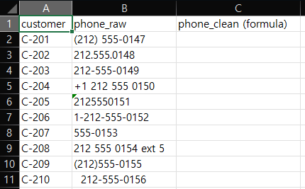
Our Phones sheet has a customer ID in column A and the raw number in column B. All values in column B are text. The ten numbers use these shapes: (212) 555-0147, 212.555.0148, 212-555-0149, +1 212 555 0150, 2125550151, 1-212-555-0152, 555-0153 (no area code), 212 555 0154 ext 5 (with an extension), (212)555-0155, and 212-555-0156 with spaces in front.

Step 1: Keep Only the Digits

In C2, enter this formula and fill it down to C11:

=SUBSTITUTE(SUBSTITUTE(SUBSTITUTE(SUBSTITUTE(SUBSTITUTE(SUBSTITUTE(B2," ",""),"-",""),"(",""),")",""),".",""),"+","")

Each SUBSTITUTE removes one character: a space, a dash, an opening parenthesis, a closing parenthesis, a dot, and a plus sign.

Most rows now hold ten digits. Three rows look different:

• +1 212 555 0150 and 1-212-555-0152 became 11 digits, because the leading 1 stayed.
• 555-0153 became 7 digits.
• 212 555 0154 ext 5 became 2125550154ext5. The formula removes only the six characters we listed, so the letters ext and the digit 5 stayed.

The spaces in front of the last number were removed too.

Step 2: Accept 10 Digits, Drop a Leading 1, Flag the Rest

Add the headers us_10digit and formatted in D1 and E1. In D2, enter:

=IF(AND(LEN(C2)=11,LEFT(C2,1)="1"),MID(C2,2,10),IF(LEN(C2)=10,C2,"CHECK"))

This returns the last ten digits if the value has 11 digits and starts with 1. If it has exactly 10 digits, it returns them unchanged. Anything else becomes CHECK.

In E2, enter:

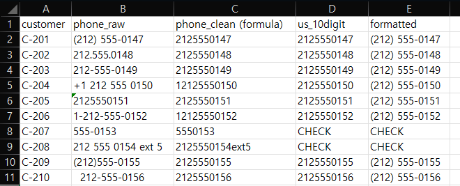
=IF(D2="CHECK","CHECK",TEXT(--D2,"(000) 000-0000"))

--D2 turns the digit text into a number, and TEXT formats it with the pattern (000) 000-0000. Microsoft’s TEXT page says the second argument defines how the value is formatted. Our pattern is not one of its examples, so the screenshot below is our evidence for it. Fill both formulas down to row 11.

The Result

Eight of the ten numbers came out as (212) 555-01xx, including the two with a leading 1 and the one with spaces in front. Two rows show CHECK in both columns:

Raw	After Step 1	Result
555-0153	5550153	CHECK (7 digits)
212 555 0154 ext 5	2125550154ext5	CHECK (letters left, not 10 or 11 digits)

Those are the numbers a person should look at. The formula does not try to guess an area code or split off the extension.

What This Formula Does Not Check

• Only length and a leading 1. A string of 10 digits passes, even if it is not a real phone number or the area code does not exist. We did not validate area codes.
• US-style numbers only. We did not test international numbers.
• Extensions. They are flagged, not parsed.
• Only ordinary spaces. The first SUBSTITUTE removes an ordinary space. If numbers copied from a web page still do not clean up, they may contain a non-breaking space, which SUBSTITUTE(B2," ","") does not match. See why TRIM isn’t removing non-breaking spaces. We did not test that character here.
• Numeric cells. Our raw column holds text. We did not test numbers stored as real numbers.
• The results are formulas and text. We did not test copying them as values.

One-line Summary

Remove the separators with nested SUBSTITUTE, keep 10 digits (or 11 with a leading 1), format them with TEXT, and let everything else show CHECK:

=IF(AND(LEN(C2)=11,LEFT(C2,1)="1"),MID(C2,2,10),IF(LEN(C2)=10,C2,"CHECK"))

Sources

• SUBSTITUTE function — Microsoft Support. Backs the Applies-to list (Microsoft 365, 2024, 2021, 2019, 2016).
• TEXT function — Microsoft Support. Backs the description of the format argument and the Applies-to list (Microsoft 365, 2024, 2021, 2019, 2016).
• Note: the digits-only results, the 8 formatted numbers, the two CHECK rows, and the (000) 000-0000 result come from our own reproduction in the Excel 2021 desktop app, not from these pages. The numbers are fictional.