Category: Text Cleanup

  • Remove Line Breaks From Cells in Excel (Ctrl+J, SUBSTITUTE, Power Query)

    Text pasted or imported into Excel can arrive with line breaks inside the cell, so one address takes three lines. This guide tries three ways to turn those breaks into spaces: Find & Replace with Ctrl+J, formulas, and Power Query. It also shows two things that went wrong in our tests, so you know what to look for.

    Tested in: Excel 2021 desktop (Home & Business 2021, Version 2608) with an English interface on Korean-language Windows. We did not test other versions or Excel for Mac.

    The Test Data

    Our LineBreaks sheet has six cells in column A. Three of them have two line breaks (two addresses and a note). Two have one line break, and one has none (No break in this one). One of the single-break cells, Line one / Line two (CRLF pasted), was created on purpose with a Windows-style line ending (a carriage return followed by a line feed). The other line breaks are a line feed only. All text is made up.
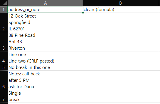
    LineBreaks sheet with six cells in column A, several showing two or three lines of text inside one cell
    Six test cells. Five contain line breaks.

    Method 1: Find & Replace With Ctrl+J

    Work on a copy of the sheet, because Replace All changes the cells in place.

    1. Select the cells, then press Ctrl+H.
    2. Click in Find what and press Ctrl+J.
    3. Put a single space in Replace with.
    4. Click Replace All.

    Excel reported “We made 8 replacements.” and every cell became a single line. Eight matches the number of line feeds in our six cells.
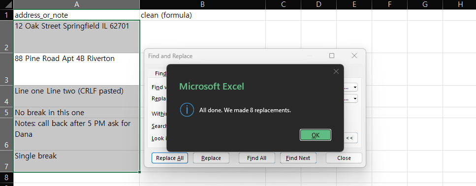
    Excel message 'All done. We made 8 replacements' above cells that now read as single lines
    Ctrl+J in Find what, a space in Replace with: 8 replacements.

    What went wrong the first time: our first Replace All said “We couldn’t find anything to replace.” The Ctrl+J had not actually been entered in the Find what box. After re-entering it, the replacement worked. We did not find out why the first attempt failed.

    We did not check whether the carriage return in the CRLF cell was still there after this method. The formulas below did check it.

    Method 2: Formulas

    We put three formulas next to the data, in columns B, C and D, and compared them:

    B2: =TRIM(SUBSTITUTE(SUBSTITUTE(A2,CHAR(13),""),CHAR(10)," "))
    C2: =SUBSTITUTE(A2,CHAR(10)," ")
    D2: =CLEAN(A2)
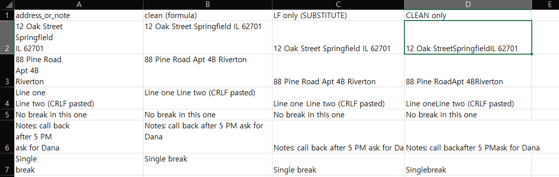
    Three formula columns next to the line-break data; the CLEAN column joins words such as StreetSpringfieldIL
    B and C look the same. D (CLEAN) removes the breaks but joins the words.

    Column B gave a clean single line on all six rows, for example 12 Oak Street Springfield IL 62701. Column C looked the same as B on screen.

    Column D, the CLEAN version, removed the line breaks but did not put a space in their place, so words ran together: 12 Oak StreetSpringfieldIL 62701 and Singlebreak. If you want readable text, use SUBSTITUTE with a space.

    Why the CRLF cell needs CHAR(13)

    B and C look identical, but they are not. We compared their lengths with =LEN(C2)-LEN(B2):

    Length-difference column showing 0, 0, 1, 0, 0, 0 for the six rows
    Only row 4, the CRLF cell, is one character longer in column C.

    The six results were 0, 0, 1, 0, 0, 0. Only row 4 (the CRLF cell) differed. Replacing only CHAR(10) left one extra invisible character in that cell. We read that as the leftover carriage return, and the CHAR(13) in column B’s formula removes it. We created that cell on purpose. We cannot say how often your data has this ending.

    Method 3: Power Query

    In Power Query, use Replace Values twice, on the text column.

    First replace the line feed with a space. In the Replace Values dialog, type #(lf) in Value To Find, expand Advanced options, and check Replace using special characters. Put a space in Replace With.

    Replace Values dialog with #(lf) in Value To Find and Replace using special characters checked under Advanced options
    Replace Values with ‘Replace using special characters’ checked.

    After this step, the CRLF row still showed two lines in the preview. Then add a second Replace Values step for #(cr), with Replace With left empty and the same checkbox checked. All six rows were then single lines:

    Power Query preview with six single-line rows after two Replace Values steps for line feed and carriage return
    Two steps, line feed to space and carriage return removed: six single lines.

    Two mistakes cost us time, and both are easy to repeat:

    • The checkbox. We typed #(cr) with Replace using special characters unchecked. The formula bar showed #(#)(cr), so Power Query searched for that text and replaced nothing. The checkbox was the likely cause, but its state was not visible in that first attempt.
    • The order. After the first step had already turned each line feed into a space, we searched for #(cr)#(lf). It matched nothing, because that pair no longer existed. Search for #(cr) alone.

    Which Method Did What

    MethodAll six rows single lineKeeps a space between linesHandles the CRLF cell
    Ctrl+J Replace AllYesYes (we typed a space)Not checked
    SUBSTITUTE CHAR(10) onlyLooks yesYesLeaves one extra character
    SUBSTITUTE with CHAR(13) and TRIMYesYesYes
    CLEAN onlyYesNo, words joinNot checked
    Power Query, two stepsYesYesYes

    Things to Know

    • Formulas leave the original alone. Columns B to D are new columns, so column A is unchanged. Find & Replace overwrites the cells.
    • Extra spaces. The TRIM in column B also removes extra ordinary spaces. TRIM does not remove non-breaking spaces; see why TRIM isn’t removing them. We did not test that character here.
    • Splitting instead. If you want the lines in separate cells instead of one line, that is a different task. We did not test it here. For splitting around one character with formulas, see extracting text before or after a character.

    One-line Summary

    Replace the line feed with a space (Ctrl+J in Find & Replace, SUBSTITUTE, or Power Query), and if your data may contain Windows-style CRLF breaks, also remove the carriage return:

    =TRIM(SUBSTITUTE(SUBSTITUTE(A2,CHAR(13),""),CHAR(10)," "))

    Sources

    • Note: every result, including the eight replacements, the length differences, and the Power Query steps, comes from our own reproduction in the Excel 2021 desktop app. We did not check these functions against Microsoft’s documentation for this guide.
  • Remove Special Characters in Excel and Keep Only Letters and Numbers

    Sometimes you want a code or a name with only letters and numbers: no dashes, hash signs, commas, or brackets. This guide does that two ways, with an Excel formula and with Power Query. It also lists what these methods remove beyond what you might expect, including spaces and accented letters.

    Tested in: Excel 2021 desktop (Home & Business 2021, Version 2608) with an English interface on Korean-language Windows. We did not test other Excel versions.

    The Test Data

    Our SpecialChars sheet has ten made-up strings in column A, such as ACME-Corp. #42!, SKU_1001/A, and A&B Co., Ltd.. Two are there to test the edges: Café Müller 12 has accented letters, and Spaced Out 9 has extra spaces. One, already_clean, contains an underscore.

    SpecialChars sheet with ten strings in column A including ACME-Corp. #42!, SKU_1001/A, Café Müller 12 and already_clean
    Ten test strings with punctuation, an accented name, extra spaces and an underscore.

    Method 1: One Formula

    In B2, enter this formula and fill it down:

    =LET(t,A2,c,MID(t,SEQUENCE(LEN(t)),1),k,CODE(c),TEXTJOIN("",TRUE,IF((k>=48)*(k<=57)+(k>=65)*(k<=90)+(k>=97)*(k<=122)>0,c,"")))

    Here is what it does:

    • MID(t,SEQUENCE(LEN(t)),1) splits the text into single characters.
    • CODE(c) gives each character’s code number.
    • The IF keeps a character only if its code is 48 to 57 (digits 0 to 9), 65 to 90 (A to Z), or 97 to 122 (a to z).
    • TEXTJOIN joins the kept characters back together.

    The formula ran without errors in our Excel 2021.

    Formula column using LET, SEQUENCE, MID, CODE and TEXTJOIN with results such as ACMECorp42 and SmithJohnVIP
    The LET formula in column B and its results.
    OriginalResult
    ACME-Corp. #42!ACMECorp42
    Smith, John (VIP)SmithJohnVIP
    SKU_1001/ASKU1001A
    100% Pure100Pure
    A&B Co., Ltd.ABCoLtd
    Order #A-77 *rush*OrderA77rush
    Cafe Muller 12CafeMuller12
    Café Müller 12CafMller12
    Spaced Out 9 SpacedOut9
    already_cleanalreadyclean

    What It Removes Besides Punctuation

    The results show three things you might not want:

    • Spaces. Every space is removed, so words join: Smith, John (VIP) becomes SmithJohnVIP.
    • Underscores and hyphens. already_clean became alreadyclean.
    • Accented letters. Café Müller 12 became CafMller12. The é and the ü are gone, not replaced by e and u.

    This follows from the rule: only A-Z, a-z, and 0-9 are kept. If you need spaces or underscores kept, the rule would have to allow more codes. We did not test a changed rule, so check any version on your own data.

    Method 2: Power Query

    In Power Query, add a custom column with this formula:

    Text.Select([raw_text], {"a".."z","A".."Z","0".."9"})

    Text.Select keeps only the characters in the list you give it. Ours was the same letters and digits.

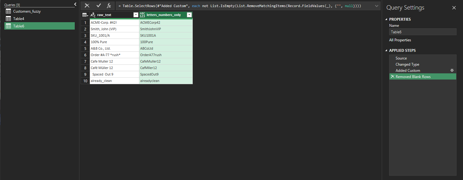
    Power Query preview with a Text.Select custom column showing ten results that match the Excel formula, including CafMller12
    Text.Select gives the same ten results as the formula.

    All ten rows matched the Excel formula, including CafMller12.

    One setup problem. Our first attempt showed 999+ rows with empty values after row 10. We had made the Power Query table from a range that was larger than the data. We fixed it by adding a Remove Blank Rows step. Selecting only the data range avoids the problem in the first place.

    Things to Know

    • Only English letters and digits are kept. Letters with accents and letters from other alphabets are removed too. We did not test a way to keep them, and we did not test any regular-expression function.
    • The formula’s code ranges. We tested it on these ten strings and did not try other character sets or other Windows language settings.
    • Original data. Both methods write to a new column, so column A is unchanged.
    • Related. If you only need to clean phone numbers, see our guide on standardizing US phone numbers. For hidden non-breaking spaces, see why TRIM isn’t removing them. We did not test either case here.

    One-line Summary

    To keep only English letters and digits, either use the LET formula above or Text.Select in Power Query. Both gave identical results on our ten strings, and both also removed spaces, underscores, hyphens, and accented letters.

    Sources

    • Note: all ten results and the Power Query comparison come from our own reproduction in the Excel 2021 desktop app. We did not check these functions against Microsoft’s documentation for this guide.
  • Extract Text Before or After a Character in Excel With LEFT, MID, and FIND

    You have an email address and want the part before the @, or the part after it. In newer Excel you can use TEXTBEFORE and TEXTAFTER. In older versions you can build the same thing from LEFT, MID, and FIND. This guide tests both on ten made-up text values and shows what each one returned, including what happened when the @ was missing and when it appeared twice.

    Applies to: Microsoft lists TEXTBEFORE for Excel for Microsoft 365 and Excel 2024. We tested in the Excel 2021 desktop app with an English interface on Korean-language Windows, so we could test only the LEFT, MID, and FIND method. We did not test other Excel versions.

    The Text

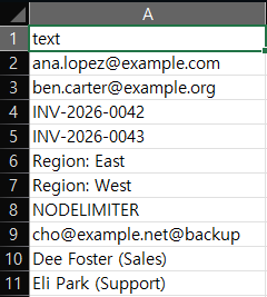
    Our Strings sheet has ten values in column A: two email addresses, two invoice codes (INV-2026-0042), two lines such as Region: East, the word NODELIMITER, an address with two @ characters (cho@example.net@backup), and two names with a department in parentheses. All values are fictional. We search for @, so only three of these values contain it. The others show what happens when the character is not there.

    Strings sheet with two email addresses, two invoice codes, two Region lines, NODELIMITER, an address with two @ and two names with departments
    Ten text values. Only three of them contain an @.

    The Classic Method: LEFT, MID and FIND

    We added the headers before_classic and after_classic in D1 and E1. In D2, enter:

    =LEFT(A2,FIND("@",A2)-1)

    In E2, enter:

    =MID(A2,FIND("@",A2)+1,100)

    Fill both down to row 11. Here is what each part does:

    • FIND("@",A2) returns the position of the first @ in the text.
    • LEFT(A2,position-1) returns everything before it.
    • MID(A2,position+1,100) returns up to 100 characters after it. The 100 is a limit we picked, so text longer than that would be cut off.
    Strings sheet with before_classic and after_classic columns: the emails are split, cho and example.net@backup, and the other rows show #VALUE!
    The LEFT/MID method splits the three @ values. The other seven rows show #VALUE!.

    The Result

    TextBefore @After @
    ana.lopez@example.comana.lopezexample.com
    ben.carter@example.orgben.carterexample.org
    cho@example.net@backupchoexample.net@backup
    INV-2026-0042, INV-2026-0043#VALUE!#VALUE!
    Region: East, Region: West#VALUE!#VALUE!
    NODELIMITER#VALUE!#VALUE!
    Dee Foster (Sales), Eli Park (Support)#VALUE!#VALUE!

    Two results are worth noting:

    • A missing character gives #VALUE!. Microsoft says FIND returns #VALUE! when it cannot find the text you ask for, and all seven rows without an @ show it. The error is not a sign that the formula is broken. It means there was nothing to split on. You could wrap the formula in IFERROR, but that hides every error, not only this one. We did not test that.
    • Two @ characters split at the first one. cho@example.net@backup returned cho before and example.net@backup after. The second @ stays in the second part. If you need the text after the last @, this formula does not do it, and we did not test a formula that does.

    What About TEXTBEFORE and TEXTAFTER?

    The newer functions do the same job in one step. We entered them in B2 and C2 of the same sheet, and filled them down:

    =TEXTBEFORE(A2,"@")
    =TEXTAFTER(A2,"@")
    Strings sheet where the TEXTBEFORE and TEXTAFTER formulas in columns B and C show #NAME? in every row
    In our Excel 2021, TEXTBEFORE and TEXTAFTER returned #NAME? in all ten rows.

    In our Excel 2021, all 20 cells showed #NAME?. Microsoft’s TEXTBEFORE page lists Excel for Microsoft 365 and Excel 2024, and Excel 2021 is not on that list. That matches what we saw. It also means we did not see how TEXTBEFORE handles a missing character or a second @, and we do not describe that here. If you get #NAME? after typing one of these functions, check your Excel version first. Our guide on splitting comma-separated values into rows covers another function that returned #NAME? in Excel 2021.

    Things to Know

    • Pick the character carefully. We searched only for @. We did not extract text around -, :, or ( in the other rows.
    • The first match only. FIND stops at the first match, as the two-@ row showed.
    • Formulas, not values. The results are formulas that depend on column A. We did not test copying them as values.

    One-line Summary

    Use LEFT with FIND for the text before a character and MID with FIND for the text after it, expect #VALUE! when the character is missing, and note that TEXTBEFORE and TEXTAFTER returned #NAME? in Excel 2021:

    =MID(A2,FIND("@",A2)+1,100)

    Sources

    • How to correct a #VALUE! error in FIND/FINDB and SEARCH/SEARCHB — Microsoft Support. Backs the statement that FIND returns #VALUE! when it cannot find the text.
    • TEXTBEFORE function — Microsoft Support. Backs the Applies-to list (Microsoft 365 and Excel 2024).
    • Note: the split results, the first-@ behavior, and the #NAME? results come from our own reproduction in the Excel 2021 desktop app, not from these pages.
  • Clean and Standardize US Phone Numbers in Excel (and Flag the Ones That Need Review)

    Phone numbers from different sources arrive in different shapes: with parentheses, dots, dashes, a leading +1, or stray spaces. You can strip them down to digits with SUBSTITUTE and then rebuild one standard format. The part that matters is what you do with the numbers that are not complete, so this guide flags those instead of guessing.

    We use ten made-up US-style numbers and show what each step returned, including the two numbers the formula refused to format.

    Applies to: Microsoft lists SUBSTITUTE and TEXT for Excel for Microsoft 365, Excel 2024, Excel 2021, Excel 2019, and Excel 2016. Tested in the Excel 2021 desktop app with an English interface on Korean-language Windows. We did not test other Excel versions. All numbers are fictional (555-01xx).

    The Raw Numbers

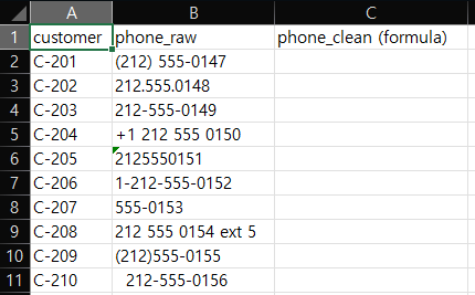
    Our Phones sheet has a customer ID in column A and the raw number in column B. All values in column B are text. The ten numbers use these shapes: (212) 555-0147, 212.555.0148, 212-555-0149, +1 212 555 0150, 2125550151, 1-212-555-0152, 555-0153 (no area code), 212 555 0154 ext 5 (with an extension), (212)555-0155, and 212-555-0156 with spaces in front.

    Phones sheet with customer IDs C-201 to C-210 and phone_raw values in ten different formats
    Ten numbers, ten shapes.

    Step 1: Keep Only the Digits

    In C2, enter this formula and fill it down to C11:

    =SUBSTITUTE(SUBSTITUTE(SUBSTITUTE(SUBSTITUTE(SUBSTITUTE(SUBSTITUTE(B2," ",""),"-",""),"(",""),")",""),".",""),"+","")

    Each SUBSTITUTE removes one character: a space, a dash, an opening parenthesis, a closing parenthesis, a dot, and a plus sign.

    Phones sheet with a phone_clean column showing digits only, including 12125550150, 5550153 and 2125550154ext5
    Only the listed characters are removed. The letters in ext 5 stay.

    Most rows now hold ten digits. Three rows look different:

    • +1 212 555 0150 and 1-212-555-0152 became 11 digits, because the leading 1 stayed.
    • 555-0153 became 7 digits.
    • 212 555 0154 ext 5 became 2125550154ext5. The formula removes only the six characters we listed, so the letters ext and the digit 5 stayed.

    The spaces in front of the last number were removed too.

    Step 2: Accept 10 Digits, Drop a Leading 1, Flag the Rest

    Add the headers us_10digit and formatted in D1 and E1. In D2, enter:

    =IF(AND(LEN(C2)=11,LEFT(C2,1)="1"),MID(C2,2,10),IF(LEN(C2)=10,C2,"CHECK"))

    This returns the last ten digits if the value has 11 digits and starts with 1. If it has exactly 10 digits, it returns them unchanged. Anything else becomes CHECK.

    In E2, enter:

    =IF(D2="CHECK","CHECK",TEXT(--D2,"(000) 000-0000"))

    --D2 turns the digit text into a number, and TEXT formats it with the pattern (000) 000-0000. Microsoft’s TEXT page says the second argument defines how the value is formatted. Our pattern is not one of its examples, so the screenshot below is our evidence for it. Fill both formulas down to row 11.

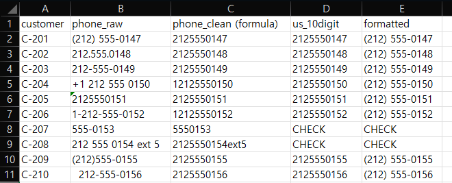
    Phones sheet with us_10digit and formatted columns: eight numbers shown as (212) 555-01xx and two rows marked CHECK
    Eight numbers are formatted. The 7-digit number and the extension row show CHECK.

    The Result

    Eight of the ten numbers came out as (212) 555-01xx, including the two with a leading 1 and the one with spaces in front. Two rows show CHECK in both columns:

    RawAfter Step 1Result
    555-01535550153CHECK (7 digits)
    212 555 0154 ext 52125550154ext5CHECK (letters left, not 10 or 11 digits)

    Those are the numbers a person should look at. The formula does not try to guess an area code or split off the extension.

    What This Formula Does Not Check

    • Only length and a leading 1. A string of 10 digits passes, even if it is not a real phone number or the area code does not exist. We did not validate area codes.
    • US-style numbers only. We did not test international numbers.
    • Extensions. They are flagged, not parsed.
    • Only ordinary spaces. The first SUBSTITUTE removes an ordinary space. If numbers copied from a web page still do not clean up, they may contain a non-breaking space, which SUBSTITUTE(B2," ","") does not match. See why TRIM isn’t removing non-breaking spaces. We did not test that character here.
    • Numeric cells. Our raw column holds text. We did not test numbers stored as real numbers.
    • The results are formulas and text. We did not test copying them as values.

    One-line Summary

    Remove the separators with nested SUBSTITUTE, keep 10 digits (or 11 with a leading 1), format them with TEXT, and let everything else show CHECK:

    =IF(AND(LEN(C2)=11,LEFT(C2,1)="1"),MID(C2,2,10),IF(LEN(C2)=10,C2,"CHECK"))

    Sources

    • SUBSTITUTE function — Microsoft Support. Backs the Applies-to list (Microsoft 365, 2024, 2021, 2019, 2016).
    • TEXT function — Microsoft Support. Backs the description of the format argument and the Applies-to list (Microsoft 365, 2024, 2021, 2019, 2016).
    • Note: the digits-only results, the 8 formatted numbers, the two CHECK rows, and the (000) 000-0000 result come from our own reproduction in the Excel 2021 desktop app, not from these pages. The numbers are fictional.
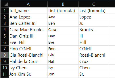
  • Split Full Names Into First and Last Name in Excel: A Simple Method and Its Limits

    A column of full names is easy to split if every name is two words. Real lists are not like that. They have middle names, suffixes such as Jr., and last names with several parts. A formula that takes the first word and the last word is quick to build, but it gets some of those names wrong.

    This guide builds that formula, runs it on ten made-up names, and shows exactly which names came out right and which did not. We also show what happened when we tried the newer TEXTBEFORE and TEXTAFTER functions in Excel 2021.

    Applies to: Microsoft lists TRIM and SUBSTITUTE for Excel for Microsoft 365, Excel 2024, Excel 2021, Excel 2019, and Excel 2016. We did not look up LEFT, RIGHT, FIND, and REPT on Microsoft’s pages. Tested in the Excel 2021 desktop app with an English interface on Korean-language Windows. We did not test other Excel versions.

    The Names

    Our Names sheet has ten full names in column A. Most are plain two-word names. The rest were chosen to cause trouble: a middle name (Cara Mae Brooks), suffixes (Ben Carter Jr., Dan Ortiz III, Jon Kim Sr.), a last name with a particle (Hal de la Cruz), a hyphenated name, a name with an apostrophe, and a name with two spaces between the words (Eve Hill). All names are fictional.

    Names sheet with ten full names including Ben Carter Jr., Cara Mae Brooks, Dan Ortiz III, Eve Hill and Hal de la Cruz
    Ten names, including a middle name, three suffixes, and de la Cruz.

    Step 1: Take the First Word

    In B2, enter this formula:

    =LEFT(TRIM(A2),FIND(" ",TRIM(A2)&" ")-1)

    Here is what each part does:

    • TRIM(A2) removes extra spaces, so the double space in Eve Hill becomes a single space.
    • FIND(" ",TRIM(A2)&" ") finds the position of the first space. We add a space at the end so the formula still works if a cell holds only one word.
    • LEFT(...,position-1) returns everything before that first space.

    Step 2: Take the Last Word

    In C2, enter this formula:

    =TRIM(RIGHT(SUBSTITUTE(TRIM(A2)," ",REPT(" ",100)),100))

    This one works in three moves. SUBSTITUTE replaces every space with 100 spaces. RIGHT(...,100) takes the last 100 characters, which is the last word surrounded by padding. TRIM removes the padding and leaves the last word.

    Fill both formulas down to row 11.

    The Result

    The formulas returned a first word and a last word for all ten rows. They were not always the right answer:

    Names with first and last word formulas: Jr., III and Sr. appear as last names, Mae and de la are missing from the results
    First and last word of each name. Jr., III and Sr. end up in the last column.
    Full nameFirstLastRight or wrong?
    Ana LopezAnaLopezRight
    Eve Hill (two spaces)EveHillRight, TRIM handled the extra space
    Finn O'NeilFinnO'NeilRight
    Gia Rossi-BianchiGiaRossi-BianchiRight
    Ivy ChenIvyChenRight
    Ben Carter Jr.BenJr.Wrong, the last name is Carter
    Dan Ortiz IIIDanIIIWrong, the last name is Ortiz
    Jon Kim Sr.JonSr.Wrong, the last name is Kim
    Cara Mae BrooksCaraBrooksIncomplete, Mae is in neither column
    Hal de la CruzHalCruzIncomplete, de la is lost

    Five names came out right and five did not. The three suffix names show the suffix as the last name, the middle name is dropped, and the particle de la is dropped from the last name. The formula cannot tell a suffix or a particle from an ordinary name, because it only counts words.

    Where This Method Breaks

    • Suffixes. Jr., III, and Sr. become the last name.
    • Middle names. The middle word is not in either column. Whether you call it a middle name or part of the first name depends on your data, and the formula does not decide.
    • Last names with several parts. de la Cruz becomes Cruz. Other multi-part names would be cut the same way.

    We did not build a formula that fixes these cases. If your list has them, one practical option is to treat any name with more than two words as a row to review by hand. We did not test a formula for that, so check it on your own data first.

    What About TEXTBEFORE and TEXTAFTER?

    Newer Excel has TEXTBEFORE and TEXTAFTER, which can split on a character without the padding trick. We tried them in the same sheet:

    =TEXTBEFORE(TRIM(A2)," ")
    =TEXTAFTER(TRIM(A2)," ",-1)
    Names sheet where the TEXTBEFORE and TEXTAFTER formulas in columns D and E show #NAME? in every row
    In our Excel 2021, TEXTBEFORE and TEXTAFTER returned #NAME? in all ten rows.

    In our Excel 2021, all ten rows in both columns showed #NAME?. Microsoft’s page for TEXTBEFORE lists Excel for Microsoft 365 and Excel 2024, and Excel 2021 is not on that list. So we do not know how these two functions handle the ten names above, and we did not compare them with the first-word and last-word formulas.

    If you see #NAME? after typing one of these functions, check your Excel version before you look for a typo. Our guide on splitting comma-separated values into rows shows another function that gave #NAME? in Excel 2021. Our guide on extracting text before or after a character shows the same #NAME? result for TEXTBEFORE and TEXTAFTER.

    Things to Know

    • Only ordinary spaces. TRIM removes ordinary spaces. Microsoft says it does not remove the non-breaking space (character 160). If a name from a web page does not split correctly, see why TRIM isn’t removing non-breaking spaces. We did not test that character here.
    • One-word names. We did not test a cell that holds only one word.
    • Original data. The formulas sit in new columns, so column A is unchanged.

    One-line Summary

    The first-word and last-word formulas split plain two-word names correctly, but they put suffixes such as Jr. in the last-name column and drop middle names and particles like de la, so review those rows by hand:

    =LEFT(TRIM(A2),FIND(" ",TRIM(A2)&" ")-1)

    Sources

    • TRIM function — Microsoft Support. Backs what TRIM removes, the note that it does not remove the non-breaking space (character 160), and the Applies-to list (Microsoft 365, 2024, 2021, 2019, 2016).
    • SUBSTITUTE function — Microsoft Support. Backs the Applies-to list (Microsoft 365, 2024, 2021, 2019, 2016).
    • TEXTBEFORE function — Microsoft Support. Backs the Applies-to list (Microsoft 365 and Excel 2024).
    • Note: the ten results, the #NAME? results for TEXTBEFORE and TEXTAFTER, and the right-or-wrong judgment for each name come from our own reproduction in the Excel 2021 desktop app, not from these pages.
  • Why TRIM Isn’t Removing Non-Breaking Spaces in Excel

    If =TRIM(A2) still leaves extra space in a cell — or two values that look identical still fail an exact-match comparison — the cause is usually a non-breaking space (NBSP, Unicode character U+00A0, decimal code 160), not a regular space. TRIM does not remove it, and one common fix formula can fail depending on your Windows language settings.

    Applies to: all current Excel versions (Excel for Microsoft 365, Excel 2024, Excel 2021, Excel 2019, Excel 2016). The CHAR(160) behavior described below was reproduced specifically on Excel 2021 running on Korean-language Windows — see the scoped explanation in the section below before assuming it applies to your setup.

    Why TRIM Alone Isn’t Enough

    Microsoft’s own documentation for the TRIM function states that the Unicode character set includes an additional space character with decimal value 160 — the non-breaking space commonly used on web pages — and that TRIM by itself does not remove this character. TRIM removes regular ASCII spaces (character code 32) from the start and end of text and collapses multiple spaces between words down to one, but it does not touch character code 160.

    This matters because non-breaking spaces commonly end up in Excel data pasted from web pages, PDFs, or other applications that use them to prevent line breaks. The cell can look completely normal — same font, same visible spacing — while LEN() reports a longer string than expected, or an exact-match formula (=A2=B2) returns FALSE for text that appears identical.

    CLEAN does not solve this either: CLEAN removes the first 32 ASCII control characters (character codes 0–31, non-printing characters like line breaks and tabs), not code 160. A non-breaking space is a printable character, not a control character, so CLEAN has no effect on it.

    TRIM formula failing to remove a non-breaking space in Excel

    The Standard Fix Formula

    The general-purpose pattern for stripping both regular and non-breaking spaces is:

    =TRIM(SUBSTITUTE(CLEAN(A2), UNICHAR(160), " "))

    Read this from the inside out:

    1. CLEAN(A2) strips any non-printing control characters.
    2. SUBSTITUTE(..., UNICHAR(160), " ") replaces every non-breaking space with a regular space.
    3. TRIM(...) then collapses the now-all-regular spaces and trims the ends.
    Full fix formula removing non-breaking spaces and matching expected text length

    A Formula That Can Fail: CHAR(160) vs. UNICHAR(160)

    A common version of this formula uses CHAR(160) instead of UNICHAR(160):

    =TRIM(SUBSTITUTE(A2, CHAR(160), CHAR(32)))

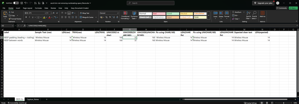
    This project reproduced one specific case where this formula did not fix the problem: on Excel 2021 running on Korean-language Windows. Direct diagnosis in Excel — checking the actual character codes in the source text with UNICODE(MID(...)), then testing =UNICODE(CHAR(160)) directly — showed that on that machine, CHAR(160) did not return the Unicode non-breaking space at all. It returned a regular space (character code 32) instead. Because CHAR(160) was returning the wrong character, SUBSTITUTE had nothing matching to replace, and the non-breaking spaces in the text were left untouched.

    On the tested machine, UNICODE(UNICHAR(160)) returned 160 while UNICODE(CHAR(160)) returned 32. That is why this article uses UNICHAR(160) for the NBSP replacement.

    CHAR(160) returning an unexpected character code on the tested Windows configuration
    UNICHAR(160) correctly returning the non-breaking space on the tested configuration

    This project has confirmed this behavior on one specific configuration (Excel 2021, Korean-language Windows) and has not tested it on other locales. It has not been verified whether this also happens on other non-Western Windows locales, other Excel versions, or other regional settings — that would require separate reproduction on each configuration. Rather than assuming the scope of the issue, the practical takeaway is: verify what CHAR(160) actually returns on your own machine before relying on it (see the check below), and default to UNICHAR(160) in any formula that needs to target the non-breaking space specifically, since it does not depend on this ambiguity.

    How to Check Whether This Affects You

    Before assuming a fix formula worked, verify it rather than trusting that it ran without an error:

    1. Check the actual character code(s) around the suspect space with =UNICODE(MID(A2, n, 1)) for the relevant position n. A non-breaking space returns 160; a regular space returns 32.
    2. Check what your own CHAR(160) actually returns: =UNICODE(CHAR(160)). If this returns 160, CHAR(160) is working correctly as a non-breaking space on your system. If it returns anything other than 160, use UNICHAR(160) instead in any formula that needs to target the non-breaking space.
    3. After applying the fix formula, re-check the result’s length with LEN() against the expected clean length, rather than assuming success because the formula didn’t error.
    UNICODE formula confirming a non-breaking space at code 160

    If the symptom you see is a lookup returning #N/A, see our guide on VLOOKUP or XLOOKUP returning #N/A on values that look identical. If you are cleaning phone numbers copied from a web page, see our guide on standardizing US phone numbers.

    One-line Summary

    TRIM alone does not remove non-breaking spaces (character code 160); use =TRIM(SUBSTITUTE(CLEAN(A2), UNICHAR(160), " ")). On at least one tested configuration (Excel 2021, Korean-language Windows), CHAR(160) returned the wrong character and silently broke a CHAR(160)-based fix formula — check what =UNICODE(CHAR(160)) returns on your own machine, and prefer UNICHAR(160) if you’re unsure.

    Sources

    • TRIM function — Microsoft Support. States that Unicode includes an additional space character (decimal value 160, the non-breaking space used on web pages) and that TRIM by itself does not remove it.
    • UNICHAR function — Microsoft Support. Backs UNICHAR’s behavior of returning the character for a given Unicode code point.
    • CLEAN function — Microsoft Support. Backs the statement that CLEAN removes the first 32 ASCII control characters and does not affect character code 160.
    • The CHAR(160) behavior — returning a regular space (code 32) instead of the non-breaking space on one specific machine (Excel 2021, Korean-language Windows), while UNICHAR(160) correctly returned code 160 on the same machine — was diagnosed and confirmed by this project through direct reproduction in Excel, recorded in the Pilot C entry of the project decision log. This is a project-verified reproduction on one configuration, not a general claim about Windows locales, and it has not been tested on other locales or Excel versions.