Replace Inconsistent Labels (USA, U.S., United States) With One Standard Value Using a Lookup Table

The same country shows up as USA, U.S., US, and United States. A PivotTable counts them as four different countries. Instead of fixing them one by one with Find and Replace, keep a small lookup table that maps every spelling to one standard value, and let a formula do the replacing.

This guide builds that table with ten made-up customers, shows the formula, and lists exactly which labels were mapped and which were not.

Applies to: Microsoft documents VLOOKUP for Excel for Microsoft 365, Excel 2024, Excel 2021, Excel 2019, and Excel 2016. Tested in the Excel desktop app with an English interface on Korean-language Windows. We did not test other Excel versions, so results may differ there.

The Messy Column

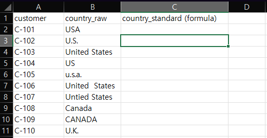
Our Labels sheet has ten customers and a country_raw column. It holds USA, U.S., United States, US, u.s.a., a United States with two spaces between the words, a typo (Untied States), Canada, CANADA, and U.K. All names are fictional.

Step 1: Build the Lookup Table

On a separate sheet (we called it CountryMap), put the spelling you see in column A and the standard value in column B. We used six rows: USA, U.S., United States, and US all point to United States, Canada points to Canada, and U.K. points to United Kingdom.

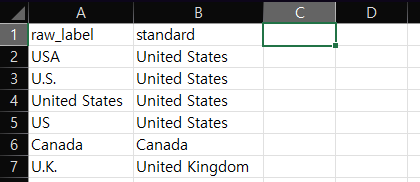
The table does not contain u.s.a., CANADA, the double-space version, or the typo. They are there on purpose, to show what the formula does with them.

Step 2: Look Up the Standard Value

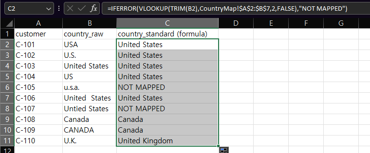
In the cell next to the first label (C2), enter this formula and fill it down to C11:

=IFERROR(VLOOKUP(TRIM(B2),CountryMap!$A$2:$B$7,2,FALSE),"NOT MAPPED")

Here is what each part does:

• TRIM(B2) removes extra spaces from the label before the lookup.
• VLOOKUP(...,2,FALSE) finds the label in column A of the table and returns the matching value from column B. FALSE asks for an exact match.
• IFERROR(...,"NOT MAPPED") shows NOT MAPPED when the label is not in the table. Without it, those rows would show #N/A.

What Happened to Each Label

Raw label	Result	Why
USA, U.S., United States, US	United States	Listed in the table
United States (two spaces)	United States	TRIM collapsed the extra space
Canada	Canada	Listed in the table
CANADA	Canada	Matched even though the case differs (our observation)
U.K.	United Kingdom	Listed in the table
u.s.a.	NOT MAPPED	Not in the table
Untied States	NOT MAPPED	A typo, not in the table

Eight of the ten rows were mapped and two were not. The NOT MAPPED text is the point of the formula: it turns a silent mistake into something you can filter for.

Microsoft’s page says leading spaces, trailing spaces, and nonprinting characters can cause unexpected VLOOKUP results. It does not say whether the match ignores case. The CANADA result is what we saw in our test, so check your own data.

How to Handle the NOT MAPPED Rows

Filter column C for NOT MAPPED and decide for each one. For u.s.a., add a new row to the table. For the typo, you can add the typo as another row in the table or fix the source value. We did not re-run the formula after changing the table. To check one list of values against another, see our guide on comparing two lists in Excel.

If you add rows to the table, make sure the formula range still covers them. Ours ended at row 7 ($A$2:$B$7).

Things to Know

• IFERROR hides every error, not only a missing label. A bad range or a broken sheet name would also show NOT MAPPED. If everything shows NOT MAPPED, check the formula first.
• TRIM does not remove non-breaking spaces. If a label with a visible space still does not map, see why TRIM isn’t removing non-breaking spaces.
• If VLOOKUP returns #N/A on values that look identical, see VLOOKUP returns #N/A when values look the same.
• We tested VLOOKUP only. We did not test XLOOKUP for this guide.

One-line Summary

Keep a two-column table of every spelling and its standard value, then use this formula and filter for NOT MAPPED to find the labels you still have to handle:

=IFERROR(VLOOKUP(TRIM(B2),CountryMap!$A$2:$B$7,2,FALSE),"NOT MAPPED")

Sources

• VLOOKUP function — Microsoft Support. Backs the exact-match behavior of FALSE, #N/A when no exact match is found, the warning about leading and trailing spaces and nonprinting characters, and the Applies-to list (Microsoft 365, 2024, 2021, 2019, 2016).
• Note: the ten-row result, the CANADA match, the two NOT MAPPED rows, and the TRIM effect on the double-space label come from our own reproduction in the Excel desktop app, not from this page.