How to Compare Two Lists in Excel (Find Missing, Extra, and Duplicate Items)

You have a master list of product codes and a list of what actually arrived. Which codes are missing, which are extra, and which appear twice? Excel can answer all three, but the answer depends on the method, because some methods ignore case or spaces and others do not.

This guide uses two short made-up lists and runs five methods on them: two COUNTIF checks, a duplicate count, a FILTER formula, and a Power Query merge. We show exactly what each one returned, including two rows that behaved differently from what you might expect.

Applies to: Microsoft lists COUNTIF, FILTER, XMATCH, and Power Query merge for Excel for Microsoft 365, Excel 2024, and Excel 2021, and TRIM also for Excel 2019 and 2016. Tested in the Excel 2021 desktop app with an English interface on Korean-language Windows. We did not test other Excel versions.

The Two Lists

Sheet ListA is the master list: 12 codes from A-101 to A-111, with A-108 entered twice. Sheet ListB is the received list: 11 codes, including a-106 in lowercase, A-105 followed by a space (we added it on purpose, and you cannot see it on screen), and the extra codes A-112 and A-113, with A-113 entered twice. All codes are fictional.

Step 1: Find Items Missing From the Other List

On ListA, in B2, enter this formula and fill it down to B13:

=IF(COUNTIF(ListB!$A$2:$A$12,A2)=0,"MISSING","ok")

COUNTIF counts how many times the code in A2 appears in the ListB range. A count of zero means the code is missing from the received list.

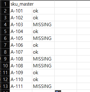
Five rows came back MISSING: A-103, A-105, both A-108 rows, and A-111. Two of those results are worth a closer look:

• A-106 was not flagged, even though ListB holds a-106 in lowercase. Microsoft says COUNTIF does not distinguish upper case from lower case, and our result agrees.
• A-105 was flagged, even though ListB appears to contain it. The ListB cell is A-105 followed by a space, so the two values are not identical. Microsoft notes that leading or trailing spaces can make COUNTIF return unexpected values.

Step 2: Find Extra Items and Trim the Spaces

Now check the other direction. On ListB, in B2, enter this formula and fill it down to B12:

=IF(COUNTIF(ListA!$A$2:$A$13,TRIM(A2))=0,"EXTRA","ok")

This time TRIM(A2) removes extra spaces from the ListB code before it is counted.

A-112 and both A-113 rows came back EXTRA. A-105 is now ok, because TRIM removed the trailing space. a-106 is ok as well.

Notice that this trimmed only the ListB value inside the formula. In Step 1 the extra space sits in ListB, so adding TRIM(A2) to the Step 1 formula would not fix it. Step 4 shows a version that trims the whole ListB range.

Step 3: Find Duplicates

On ListA, in C2, enter this formula and fill it down to C13:

=COUNTIF($A$2:$A$13,A2)

Each cell now shows how many times its own code appears in the list. We also used Conditional Formatting > Highlight Cells Rules > Duplicate Values on column A to color the repeated codes.

Both A-108 rows show 2 and are highlighted. Every other code shows 1. We checked duplicates in the master list only.

Step 4: Get the Differences as a List

Instead of flags next to each row, you can have Excel return the missing codes as a list. On a new sheet (we called it Result), enter this in A2:

=FILTER(ListA!A2:A13,ISNA(XMATCH(ListA!A2:A13,TRIM(ListB!A2:A12))))

Here is what each part does:

• TRIM(ListB!A2:A12) removes extra spaces from every code in the received list.
• XMATCH(...) looks up each master code in the trimmed list. A code that is not found returns #N/A.
• ISNA(...) turns each #N/A into TRUE.
• FILTER(...) keeps the master codes where the answer is TRUE, and the results spill down the sheet.

The result has four rows: A-103, A-108, A-108, and A-111. A-105 is not listed, because the trim removed the space. A-106 is not listed either, so XMATCH ignored the difference in case in our test. The duplicate A-108 is kept, so it shows up twice. Microsoft lists FILTER and XMATCH for Excel for Microsoft 365, Excel 2024, and Excel 2021. We did not test older versions.

Step 5: Compare With Power Query

Power Query can do the same comparison with a merge. In our test it was stricter than the formulas above.

1. Select the master list on ListA, then choose Data > From Table/Range. In the Create Table box, check My table has headers, then click OK.
2. In the Power Query Editor, choose Home > Close & Load To… > Only Create Connection.
3. Repeat for ListB.
4. Choose Data > Get Data > Combine Queries > Merge. Pick the master query on top and the received query below, click the code column in each preview, and set Join Kind to Left Anti (rows only in first). Click OK.

Microsoft describes a left anti join as bringing in only the rows from the primary table that have no matching row in the related table. That is the “missing from the other list” check.

The merge returned six rows: A-103, A-105, A-106, A-108 (twice), and A-111. Compare that with the FILTER result. A-105 and A-106 are in the list, because in our test the merge did not treat A-105 with a trailing space or lowercase a-106 as the same as the master codes. We did not use any cleaning step or case option, so we cannot say what every setting would do.

If you set up this merge and My table has headers is unchecked, Excel names the column Column1 and turns the header text into a data row. We did that on our first try, and the header text showed up in the result as if it were a code.

Which Method to Use

Method	What it returns	Case and spaces in our test
COUNTIF flag (Steps 1 and 2)	A flag next to each row, in either direction	Case ignored. A trailing space prevented a match until we added TRIM.
COUNTIF count (Step 3)	How many times each code appears	Not tested for case or spaces.
FILTER + XMATCH + TRIM (Step 4)	A list of the missing codes	Case ignored. The trailing space was trimmed. Duplicates kept.
Power Query Left Anti (Step 5)	A table of the missing codes	a-106 and A-105 were not matched. Duplicates kept.

If you only need to see the problem rows, use the flags. If you need a list to send to someone, use FILTER or the merge, and decide first whether case and spaces should count as differences.

What These Tests Do Not Cover

• Only ordinary spaces. TRIM removes ordinary spaces. Microsoft says it does not remove the non-breaking space (character 160). We did not test that character here. If a code still does not match after TRIM, see why TRIM isn’t removing non-breaking spaces. For a lookup that returns #N/A on values that look the same, see VLOOKUP returns #N/A when values look identical.
• Other versions and settings. We did not test Excel 2019 or earlier, XLOOKUP, or any case option in Power Query.
• Other data. We used text codes only. Numbers stored as text, longer lists, and lists with more than one difference per row were not tested.
• Removing duplicates. This guide finds them. To remove them, see removing duplicates with Power Query.

One-line Summary

Use COUNTIF flags to see missing and extra codes, COUNTIF counts to see duplicates, and FILTER with XMATCH and TRIM to list the differences, and check your own data for case and spacing before you trust a merge:

=FILTER(ListA!A2:A13,ISNA(XMATCH(ListA!A2:A13,TRIM(ListB!A2:A12))))

Sources

• Use the COUNTIF function — Microsoft Support. Backs the statement that COUNTIF does not distinguish case, the note on leading or trailing spaces and nonprinting characters, and the Applies-to list (Microsoft 365, 2024, 2021).
• FILTER function and XMATCH function — Microsoft Support. Back the Applies-to lists (Microsoft 365, 2024, 2021).
• TRIM function — Microsoft Support. Backs what TRIM removes, the note that it does not remove the non-breaking space (character 160), and the Applies-to list (Microsoft 365, 2024, 2021, 2019, 2016).
• Merge queries (Power Query) — Microsoft Support. Backs the description of a left anti join and the Applies-to list (Microsoft 365, 2024, 2021). The page does not say whether merge matching is case sensitive.
• Note: the MISSING, EXTRA, and count results, the FILTER output, the six-row merge result, and the a-106 and A-105 behavior come from our own reproduction in the Excel 2021 desktop app, not from these pages.