Fill Blank Cells With the Value Above in Excel (Grouped Report Exports)

Many report exports print a group label once and leave the cells below it empty. Sorting, filtering, or a PivotTable then treats those empty cells as missing data. You can fill each blank with the value above it in a few steps, without copying anything by hand.

This guide uses a small made-up sales list, selects only the blank cells, and fills them with one formula. We also point out what we did not test.

Applies to: Microsoft documents Go To Special and its Blanks option for Excel for Microsoft 365, Excel 2024, and Excel 2021. Tested in the Excel desktop app with an English interface on Korean-language Windows. We did not test other Excel versions, so menu names may differ.

What the Export Looks Like

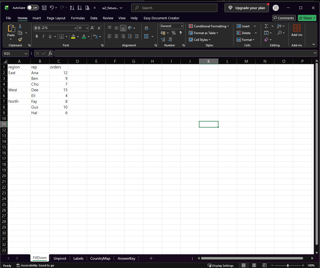
Our test sheet has three columns: region, rep, and orders. The region is filled only on the first row of each group (East in row 2, West in row 5, and North in row 7). The cells below each one are empty. All names and numbers are fictional.

Step 1: Select Only the Blank Cells

Select the cells of the region column that hold the data. Then open the Go To dialog (Home > Find & Select > Go To, or press Ctrl+G), click Special, choose Blanks, and click OK.

Excel now has only the empty cells selected. The cells that already hold a region are not part of the selection.

Step 2: Type the Formula and Fill All Blanks at Once

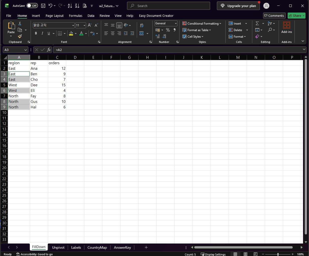
Do not click anywhere yet. The first selected blank cell is the active cell. Type a formula that points to the cell directly above it. In our sheet the first blank cell was A3, so we typed this:

=A2

Then press Ctrl+Enter instead of Enter. Excel enters the formula in every selected cell, and each one points to the cell above it.

The Result

Every blank now shows the value above it: East three times, West twice, and North three times. Cell A3 holds =A2, as the formula bar shows. The status bar counted 5 filled cells, which matches the five blanks we started with.

Check These Before You Rely on It

• The cells are formulas, not values. We did not test converting them to values, so check that before you sort or copy the column somewhere else.
• The formula copies whatever is above. If a blank cell is a real gap and not the continuation of a group, it will be filled too. Scan your data first.
• Cells that look empty may not be selected. If Blanks does not select a cell that looks empty, it may contain an empty string. Our guide on Power Query null vs empty string explains the difference. If you want to delete empty rows instead, see removing blank rows without breaking formulas.
• We tested a single column. We did not try several columns at once, a filtered list, or a Power Query Fill Down step.

One-line Summary

Select the column, use Go To > Special > Blanks, type =A2 (a reference to the cell above the first blank), and press Ctrl+Enter.

Sources

• Find and select cells that meet specific conditions — Microsoft Support. Backs the Home > Find & Select > Go To > Special path, the Blanks option (“Blank cells”), the Ctrl+G shortcut, and the Applies-to list (Microsoft 365, 2024, 2021).
• Note: the =A2 formula, the Ctrl+Enter fill, the East/West/North result, and the Count: 5 status bar come from our own reproduction in the Excel desktop app, not from this page.