Category: Power Query

  • ISO 8601 Timestamps in Excel: Handle Time Zone Offsets Safely With Power Query

    An ISO 8601 timestamp looks like 2026-03-05T14:30:00Z or 2026-03-05T23:30:00+09:00. The ending tells you which time zone the clock time belongs to. Exports from apps, logs, and APIs often use this format.

    The risk in Excel is that the ending can be dropped or reinterpreted on the way in, and the cell then shows a time that no longer matches the moment in the file. This guide shows what we observed on one test file, and how Power Query’s DateTimeZone.ToUtc lined the values up.

    Tested in: Excel 2021 desktop (Version 2608) with an English interface, Windows time zone (UTC+09:00) Seoul. Screenshots were captured in Excel 2021 with an English interface on Windows using Korean regional settings; time values may display with Korean AM/PM markers. We did not test other time zones, other Excel versions, or Mac, and results may differ there.

    Our Test File

    The CSV has five moments, each written four ways in four columns:

    ColumnExample (first row)
    ts_utc_z2026-03-05T14:30:00Z
    ts_offset_plus92026-03-05T23:30:00+09:00
    ts_offset_minus052026-03-05T09:30:00-05:00
    ts_no_zone2026-03-05T14:30:00

    The first three columns are the same instant. ts_no_zone has the same digits as the Z column but no ending at all.

    Opening the CSV by Double-Click

    When we double-clicked the file, all four columns arrived as left-aligned text, with the T and the endings kept exactly as written.
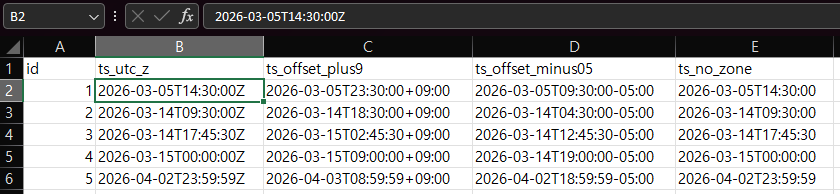
    CSV opened in Excel with four ISO 8601 timestamp columns left-aligned as text, cell B2 showing 2026-03-05T14:30:00Z
    Opened by double-click: the ISO strings stay as text.

    In this test, ISO strings containing a T stayed as text when opened by double-click.

    Importing With Data > From Text/CSV

    When we imported the same file with Data > From Text/CSV and opened Transform Data, Power Query had added a Changed Type step on its own:

    Power Query Editor with an automatic Changed Type step; the ts_utc_z column shows 2026-03-05 11:30:00 PM for a file value of 14:30Z
    Automatic Changed Type: the Z column shows 11:30 PM for a file value of 14:30Z.

    The result differed by column:

    • ts_utc_z became a date-time and showed 11:30:00 PM for the file value 14:30:00Z, nine hours later than the file.
    • ts_offset_plus9 and ts_offset_minus05 became date-time-zone values and kept their offsets (+09:00, -05:00).
    • ts_no_zone became a plain date-time and showed 2:30:00 PM, unchanged.

    We did not investigate why the Z column moved while the offset columns did not. Microsoft’s documentation says Power Query detects data types automatically for CSV files, based on the first 200 rows. The point for you is that a type step you did not write can change what a column means, so check it.

    Reading the Text Yourself With DateTimeZone.FromText

    To control the conversion, we wrote our own query that reads the columns as text and parses each one with DateTimeZone.FromText. Now the offsets were visible and the Z column read as +00:00, with no nine-hour shift:

    Power Query Editor after DateTimeZone.FromText showing +00:00, +09:00, and -05:00 offsets on the timestamp columns
    After DateTimeZone.FromText: each value carries its offset.

    Look at ts_no_zone. It has no ending in the file, but Power Query showed it as 2:30:00 PM +09:00. In our test, a string with no time zone was read as being in this PC’s time zone, which is Seoul. Keep that in mind for the conversion below.

    What Happens When You Load It to a Sheet

    We loaded this parsed query to a worksheet. The offsets did not come along. The cells show only a date and a time, with no time zone label:
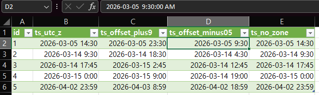
    Worksheet table with timestamp columns showing no time zone labels; the same instant appears as 14:30, 23:30, and 9:30 in different columns
    On the sheet, the offset is gone: one instant shows as 14:30, 23:30, and 9:30.

    In row 1, the Z column shows 14:30, the +09:00 column shows 23:30, and the -05:00 column shows 9:30, though all three are the same instant. The ts_no_zone column also shows 14:30, which looks identical to the Z column even though Power Query had read it as +09:00.

    Microsoft’s Power Query documentation says a date-time-zone value is converted to a date-time when loaded into the model. We observed the same loss when loading to a worksheet table. We only tested Excel 2021 with a Seoul time zone, so we can only say it can happen, not that it always does.

    Line Them Up in UTC

    The fix is to convert every value to one reference time zone before it reaches the sheet. We used three steps after the header row is promoted:

    1. DateTimeZone.FromText reads each string into a date-time-zone value.
    2. DateTimeZone.ToUtc converts each one to UTC.
    3. DateTimeZone.RemoveZone drops the zone label, so the column loads cleanly as a plain date-time that is known to be UTC.

    Note: in our test (Excel 2021, Windows time zone UTC+09:00 Seoul), a column with no time zone ending was read as +09:00, which matches the PC’s time zone. We did not test other time zones, so confirm which zone the data was written in before using the result.

    This code is an example for our five-column test CSV, not a general import. Two settings in the first line limit it. Columns = 5 makes Power Query read five columns; according to Microsoft’s documentation, extra columns in a wider file are ignored, so you could lose data without an error, and missing columns are added empty. QuoteStyle = QuoteStyle.None treats every line break as the end of a row, even inside a quoted value. Our test file has no quoted fields, so that is safe here. If your file has quoted text that contains line breaks, remove that option, because the default, QuoteStyle.Csv, keeps quoted line breaks as part of the value. We did not test files like that, or files with a different number of columns.

    let
        Source = Csv.Document(File.Contents("C:\Path\To\your-file.csv"), [Delimiter = ",", Columns = 5, Encoding = 65001, QuoteStyle = QuoteStyle.None]),
        Promoted = Table.PromoteHeaders(Source, [PromoteAllScalars = true]),
        Parsed = Table.TransformColumns(Promoted, {
            {"ts_utc_z", each DateTimeZone.FromText(_), type datetimezone},
            {"ts_offset_plus9", each DateTimeZone.FromText(_), type datetimezone},
            {"ts_offset_minus05", each DateTimeZone.FromText(_), type datetimezone},
            {"ts_no_zone", each DateTimeZone.FromText(_), type datetimezone}}),
        ToUtc = Table.TransformColumns(Parsed, {
            {"ts_utc_z", each DateTimeZone.ToUtc(_), type datetimezone},
            {"ts_offset_plus9", each DateTimeZone.ToUtc(_), type datetimezone},
            {"ts_offset_minus05", each DateTimeZone.ToUtc(_), type datetimezone},
            {"ts_no_zone", each DateTimeZone.ToUtc(_), type datetimezone}}),
        UtcNoZone = Table.TransformColumns(ToUtc, {
            {"ts_utc_z", each DateTimeZone.RemoveZone(_), type datetime},
            {"ts_offset_plus9", each DateTimeZone.RemoveZone(_), type datetime},
            {"ts_offset_minus05", each DateTimeZone.RemoveZone(_), type datetime},
            {"ts_no_zone", each DateTimeZone.RemoveZone(_), type datetime}})
    in
        UtcNoZone

    Replace C:\Path\To\your-file.csv with the full path to your CSV file, and replace the column names with your own. In Power Query, you can paste this into Home > Advanced Editor.

    Here is the ToUtc step. The first three columns show the same value in each row, +00:00. The ts_no_zone column, selected, shows a different one:

    Power Query Editor with DateTimeZone.ToUtc applied, showing UTC results for timestamp columns and the ts_no_zone column highlighted
    After ToUtc: three columns match; ts_no_zone shows 5:30 AM where the others show 2:30 PM.

    In row 1, the three real-offset columns show 2:30:00 PM +00:00. The ts_no_zone column shows 5:30:00 AM +00:00, nine hours earlier. This follows from the earlier step: the string was read as Seoul time, so converting it to UTC moved it back nine hours.

    After loading the finished query, the sheet shows the three columns with matching values:

    Worksheet table where ts_utc_z, ts_offset_plus9, and ts_offset_minus05 show identical date-times while ts_no_zone shows earlier times
    Loaded to the sheet: three columns now match; ts_no_zone differs.

    Row 1 reads 2026-03-05 14:30 in all three, and the later rows match as well (9:30, 17:45, 0:00, 23:59).

    Microsoft’s pages describe the functions this way: DateTimeZone.ToUtc “changes timezone information of the datetime value … to the UTC”. DateTimeZone.RemoveZone returns a date-time with the time zone information removed. Their FromText page shows ISO 8601 strings with numeric offsets such as -08:00; it does not mention a trailing Z, and the Z reading above is what we observed.

    Strings With No Time Zone

    The ts_no_zone column is the risky one. Excel cannot know which zone the writer meant. In our test it was read as Seoul time, so it landed nine hours away from the same-looking Z column. If those strings were really written in UTC, treating them as local would be wrong. Ask whoever produced the file which zone they meant before you convert. We did not test how to force a different assumed zone, so this guide does not cover it.

    Things to Know

    • Scope. Everything above is from one test file on Excel 2021 with a Seoul time zone. Results can differ with another time zone or Excel version, and we did not test Mac.
    • After RemoveZone. The sheet cells no longer say they are UTC, so label the column or sheet.
    • Dates only. If your values are plain dates, see fixing dates after a CSV import. For splitting a date-time that is already text, see splitting date and time in one cell.

    One-line Summary

    Before loading ISO 8601 timestamps with Z or an offset into a sheet, parse them with DateTimeZone.FromText, convert with DateTimeZone.ToUtc, and drop the label with DateTimeZone.RemoveZone, because in our Excel 2021 / Seoul test the sheet kept no offset.

    Sources

  • Find Near-Duplicate Names in Excel With Power Query Fuzzy Matching

    Removing exact duplicates is easy. Jon Smith and John Smith are not exact duplicates, so a normal duplicate check keeps both. Power Query has a fuzzy merge that can pair up names that are similar but not identical.

    This guide merges a customer list with itself using fuzzy matching and filters out each row’s match with itself. What is left is a list of candidate pairs. We ran it on 18 made-up names and report what it paired, what it missed, and what changed when we lowered the similarity threshold. The result is a candidate list for a person to review, not a final answer.

    Tested in: Excel 2021 desktop (Home & Business 2021, Version 2608) with an English interface on Korean-language Windows. We did not test other Excel versions.

    The List

    Our Customers sheet has one column, customer_name, with 18 names. They include a pair that differs by one letter (Jon Smith, John Smith), a spelling variant (Katherine Lee, Catherine Lee), an exact duplicate (Priya Patel twice), a nickname (Mike Johnson, Michael Johnson), a company name written two ways (Acme Corp, ACME Corporation), a double space (Maria Garcia, Maria Garcia), and two names that may be different people (Dan Brown, Dana Brown). All names are fictional.

    Customers sheet with 18 names in one column, including Jon Smith, John Smith, Priya Patel twice, Acme Corp and ACME Corporation
    18 names in one column. Some are near-duplicates, some are exact duplicates.

    Step 1: Add an Index Column

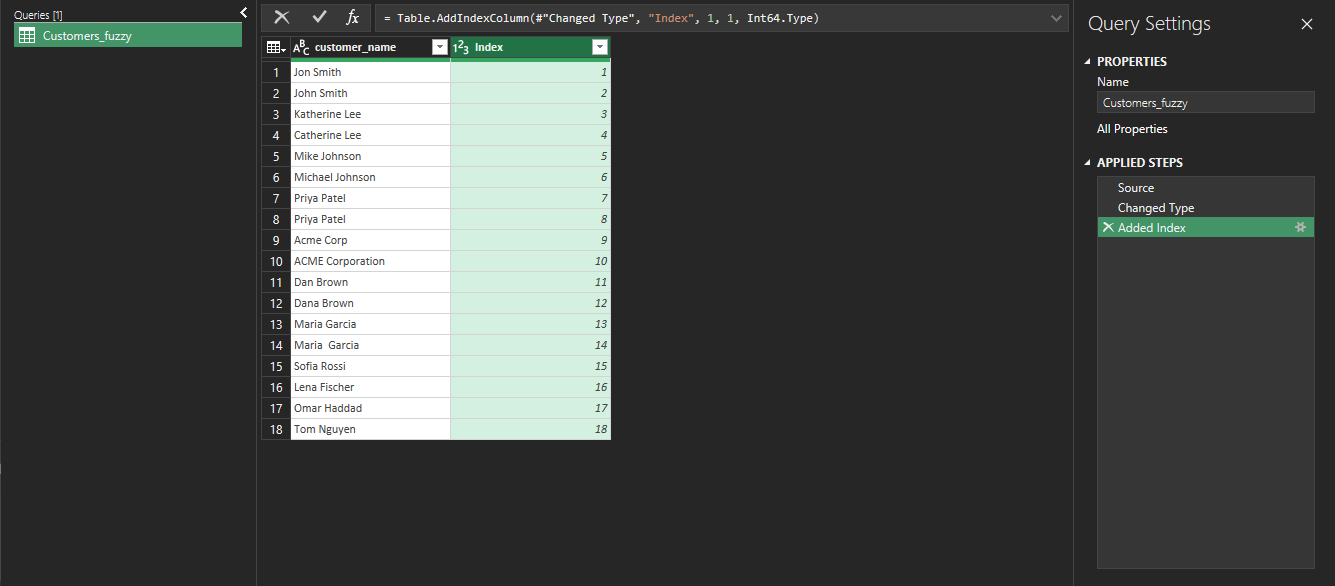
    Load the list into Power Query (select a cell in the list, then Data > From Table/Range). Then add an index column that starts at 1 (Add Column > Index Column > From 1). Our query got a second column called Index with the numbers 1 to 18.

    Power Query editor showing customer_name and an Index column numbered 1 to 18
    The Index column gives every row a number.

    The index matters later. When a list is merged with itself, every name matches itself. The index lets us remove those self-matches.

    Step 2: Merge the Query With Itself

    Choose Home > Merge Queries. In the dialog, the second table can be the same query: ours was listed as Customers_fuzzy (Current). Select customer_name in both tables, set Join Kind to Inner, and check Use fuzzy matching to perform the merge.

    Merge dialog with the same query selected twice, customer_name chosen in both tables, Inner join and fuzzy matching checked
    The same query merged with itself, with fuzzy matching on.

    The fuzzy options in our dialog were: Similarity threshold (optional), Ignore case, Match by combining text parts, Maximum number of matches (optional), and Transformation table (optional). We left the similarity threshold blank for the first run. The screen does not show what default value Power Query uses in that case, so we do not state one.

    Step 3: Expand and Remove Self-Matches

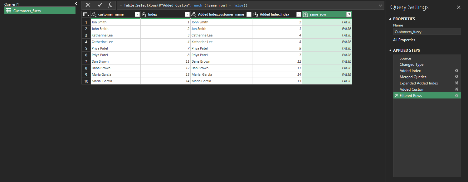
    Expand the new column and keep both customer_name and Index. Power Query names them Added Index.customer_name and Added Index.Index. Then add a custom column named same_row with this formula:

    [Index] = [Added Index.Index]

    Filter same_row to keep only FALSE. A TRUE row is a name matched with itself.

    The Result With the Default Threshold

    With the threshold blank, the result had 10 rows. Each pair appears twice, once in each direction, so that is 5 pairs:

    Power Query result with 10 rows pairing Jon Smith and John Smith, Katherine and Catherine Lee, Priya Patel twice, Dan and Dana Brown, and Maria Garcia
    Default threshold: 10 rows, which is 5 pairs counted in both directions.
    PairKind of difference
    Jon Smith and John SmithOne letter
    Katherine Lee and Catherine LeeSpelling variant
    Priya Patel and Priya PatelExact duplicate
    Dan Brown and Dana BrownPossibly two different people
    Maria Garcia and Maria GarciaDouble space

    Two pairs we expected were not in the list: Mike Johnson with Michael Johnson, and Acme Corp with ACME Corporation.

    What Happened When We Changed the Threshold

    We ran the same steps with three thresholds typed into the Similarity threshold box:

    ThresholdRowsPairsDifference
    blank (default)105Mike/Michael and Acme/ACME missing
    0.6105Same 5 pairs
    0.9105Same 5 pairs
    0.3147Adds Mike/Michael and Acme/ACME

    Going from the default to 0.6 or 0.9 changed nothing on this list. At 0.3 the two missing pairs appeared, and no unrelated names such as Sofia Rossi or Omar Haddad were paired with them.

    Power Query result with 14 rows at threshold 0.3, now including Mike Johnson and Michael Johnson and Acme Corp and ACME Corporation
    Threshold 0.3: 14 rows, 7 pairs. Mike/Michael and Acme/ACME are now included.

    Dan Brown and Dana Brown were paired at every threshold we tried. A threshold does not tell you whether two similar names are the same person. That takes a person who can look at an address, an email, or an order history.

    Load the Candidate Pairs

    Choose Close & Load to put the pairs on a new sheet. With the 0.3 threshold, our sheet had 14 rows of pairs, and the original Customers sheet was unchanged.

    New worksheet listing 14 rows of name pairs with customer_name, Index and same_row columns
    The loaded candidate list: 14 rows, 7 pairs counted in both directions.

    Things to Know

    • One small test. This is one run on 18 names. We do not know how the same settings behave on other data, and we did not test a large list.
    • We cannot explain the misses. We saw that Mike Johnson and Acme Corp were not paired at the default, 0.6, or 0.9. We did not find out why.
    • Not tested. We did not use Maximum number of matches or a Transformation table.
    • Whitespace. The double-space pair was matched. For ordinary spaces and the non-breaking space, see why TRIM isn’t removing non-breaking spaces. We did not test that character here.
    • Exact duplicates. If you only need exact duplicates, Power Query’s Remove Duplicates is the simpler tool. To find items that are in one list and not in another, see comparing two lists.

    One-line Summary

    A fuzzy merge of a list with itself, minus the self-matches, gives a candidate list of near-duplicate names for a person to review. On our 18 names it found 5 pairs by default and 7 pairs at a threshold of 0.3, and it paired Dan Brown with Dana Brown at every threshold.

    Sources

    • Note: every result in this guide, including the pairs, the thresholds, and the formulas shown in the editor, comes from our own reproduction in the Excel 2021 desktop app. We did not check the fuzzy merge options against Microsoft’s documentation, so we make no claim about how the similarity score is calculated.
  • Unpivot Columns to Rows in Excel With Power Query

    A report with one column per month is easy to read but hard to sort, filter, or summarize. Power Query can turn those month columns into rows, so each value gets its own line with the month name next to it.

    This guide uses a made-up table with one product per row and three month columns. We unpivot it, show the exact result, and point out what happened to the one empty cell.

    Applies to: Microsoft documents unpivoting columns in Power Query for Excel for Microsoft 365, Excel 2024, and Excel 2021. Tested in the Excel desktop app with an English interface on Korean-language Windows. We did not test other Excel versions, so menu names may differ.

    What the Data Looks Like

    Our test sheet has a product column and one column each for Jan, Feb, and Mar. Three products, nine numbers, except that the Gadget cell under Feb is empty. All names and numbers are fictional.

    Wide worksheet with product and Jan, Feb, Mar columns; the Gadget Feb cell is empty
    One column per month. The Gadget cell under Feb is empty.

    Step 1: Send the Table to Power Query

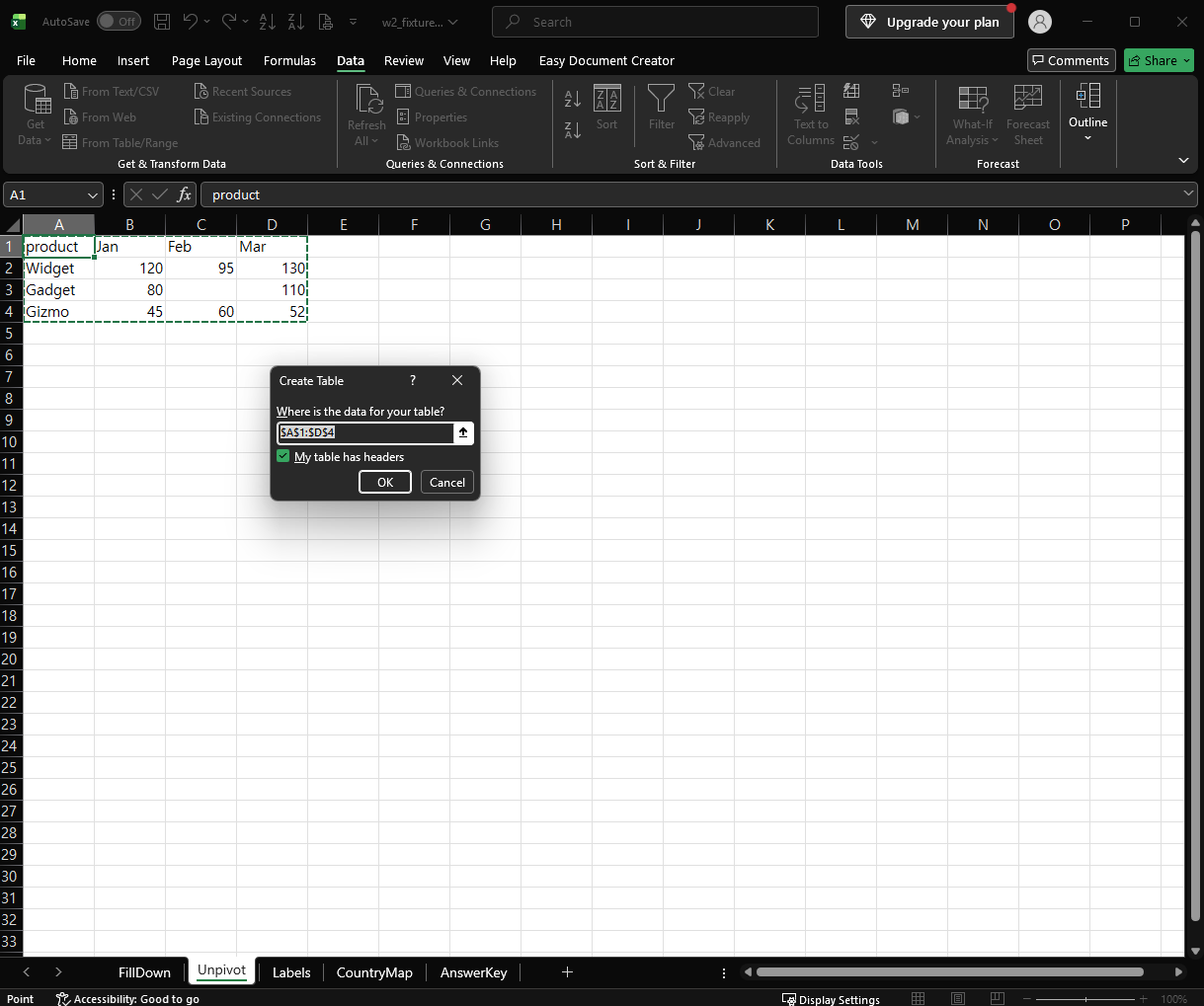
    Click any cell in the data. On the Data tab, choose From Table/Range. Excel asks you to confirm the range and whether the table has headers.

    Create Table dialog for the range A1:D4 with the table-has-headers option checked
    Confirm the range and the header option, then click OK.

    We confirmed A1:D4 with the header option checked. The Power Query Editor opens with the data and a Changed Type step. Excel named our query Table2, and yours may have another name.

    Step 2: Unpivot the Other Columns

    Click the product column header to select it. On the Transform tab, open the Unpivot Columns drop-down. It has three commands: Unpivot Columns, Unpivot Other Columns, and Unpivot Only Selected Columns.

    Power Query Transform tab with the Unpivot Columns menu open showing Unpivot Other Columns
    Select product, then choose Unpivot Other Columns.

    Choose Unpivot Other Columns. This keeps the column you selected and turns every other column into rows. Per Microsoft, it is the command to use when you do not know all the column names in advance.

    The Result

    The table now has three columns: product, Attribute (the old column names), and Value (the numbers). It has 8 rows. The step list shows Source, Changed Type, and Unpivoted Other Columns, and the step uses this formula:

    = Table.UnpivotOtherColumns(#"Changed Type", {"product"}, "Attribute", "Value")
    Unpivoted result with product, Attribute and Value columns, 8 rows, and Unpivoted Other Columns step
    The unpivoted table: 3 columns and 8 rows. There is no row for Gadget in Feb.

    We started with nine value cells and got eight rows. The empty Gadget / Feb cell did not become a row. In the preview the empty cell had shown as null, and the unpivoted result has no line for it. Check this if you count rows or total the values afterward.

    If you need a row for the empty cell, replace the null with a value before you unpivot. We did not test that.

    What We Did Not Test

    • Loading the result back to a worksheet with Close & Load.
    • Adding a new month column and refreshing. Microsoft says new columns are also unpivoted when you use Unpivot Other Columns. We did not verify that ourselves.
    • Tables with more than one ID column, text values in the month columns, or other Excel versions.

    For background on what a null is, see our guide on null vs empty string in Power Query. Another way to reshape data into rows is covered in splitting comma-separated values into rows.

    One-line Summary

    Use Data > From Table/Range, select the ID column, choose Transform > Unpivot Columns > Unpivot Other Columns, and check the row count, because empty cells do not become rows.

    Sources

    • Unpivot columns (Power Query) — Microsoft Support. Backs the Transform tab commands, what each of the three commands does, the statement that Unpivot Other Columns suits unknown column names, the statement that new columns added during a refresh are also unpivoted, and the Applies-to list (Microsoft 365, 2024, 2021).
    • Note: the 8-row result, the missing Gadget / Feb row, the Table.UnpivotOtherColumns formula, and the Create Table step come from our own reproduction in the Excel desktop app, not from this page.
  • Combine Multiple CSV Files From a Folder With Power Query (and Keep It Refreshable)

    You get one CSV per month and you need them in one table. Copy and paste works once, and then next month you do it again. Power Query can read every file in a folder and stack them into one table that you refresh when a new file arrives.

    This guide shows the whole path with four small test files, one of which has a different column order and one of which has a changed header and a blank line. The combined result was not what we first expected, so you will also see what went wrong, how we fixed it, and how a new file showed up after a refresh.

    Applies to: Microsoft documents importing a folder of files with Power Query for Excel for Microsoft 365, Excel 2024, Excel 2021, Excel 2019, and Excel 2016. Tested in the Excel desktop app with an English interface on Korean-language Windows. We tested CSV files only and did not test other Excel versions, so menu names may differ.

    The files are made up: sales_2026-01.csv to sales_2026-04.csv, each with order_id, region, product, qty, and unit_price. The February file lists the same columns in a different order. The March file calls the first column Order ID and has a blank line after its first row. All values are fictional.

    Step 1: Put the Files in One Folder

    Put the CSV files in a folder by themselves. Microsoft says every file in the folder and its subfolders is included, and that the files should have matching column headers, data types, and column count. Column order can differ, because Power Query matches columns by name.

    Do not save your workbook in that folder. Any other file in the folder would be listed too.

    Step 2: Point Excel at the Folder

    On the Data tab, choose Get Data > From File > From Folder, and select the folder. Excel lists the files it found.

    Power Query folder file list showing four sales CSV files with Combine, Load and Transform Data buttons
    The folder dialog lists the four CSV files. Choose Combine to merge them.

    We saw four files and three buttons: Combine, Load, and Transform Data. Transform Data only opens the list of files. It does not merge them. To merge, use Combine.

    Step 3: Combine

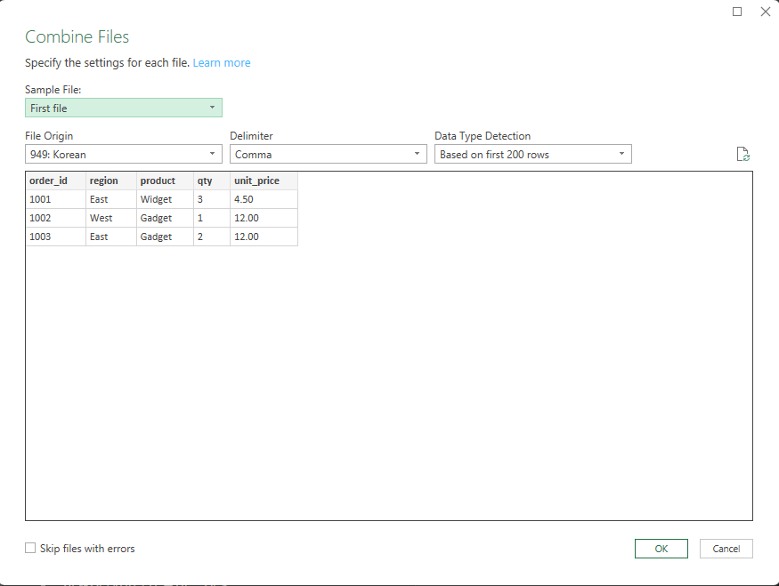
    Click Combine and then Combine & Transform Data. The Combine Files dialog asks which file to use as the sample and how to read it.

    Combine Files dialog: First file as sample, Comma delimiter, preview with order_id, region, product, qty, unit_price
    The Combine Files dialog. We left every setting as it was.

    On our computer the dialog showed First file as the sample, Comma as the delimiter, and Based on first 200 rows for data type detection. File Origin was set to 949: Korean, which matches our Korean-language Windows. We did not change any setting. If your files use another encoding, check this box.

    Click OK. The Power Query Editor opens with the combined table.

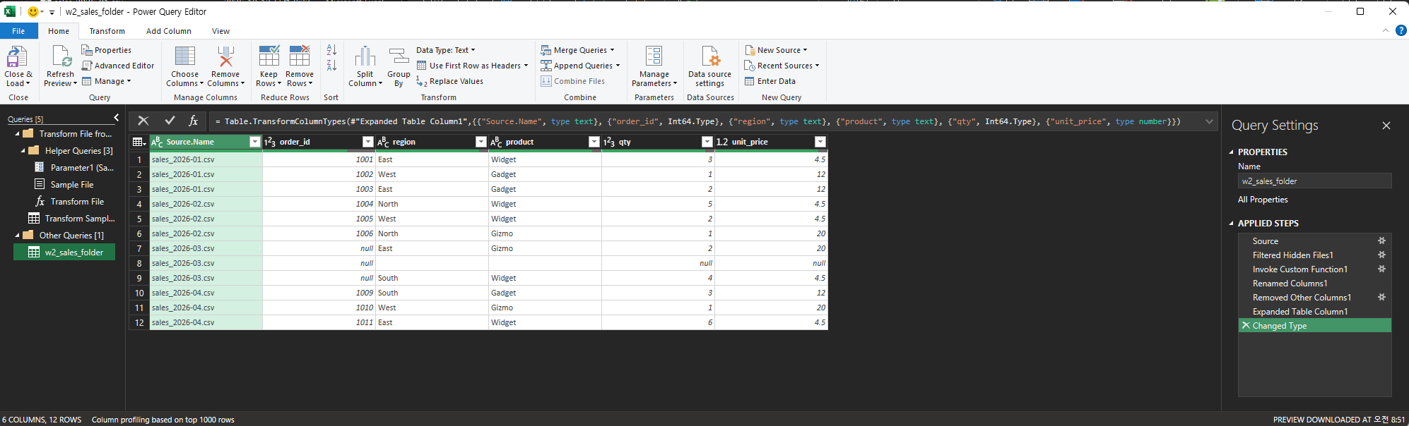
    Power Query result of the combined folder: 6 columns and 12 rows with Source.Name and the Applied Steps list
    The first combined result: 6 columns and 12 rows.

    The result had 6 columns and 12 rows. Power Query added a Source.Name column that shows which file each row came from. On the left it created helper queries (Sample File, Parameter1, Transform File, and Transform Sample File), and the main query ended with these steps: Source, Filtered Hidden Files1, Invoke Custom Function1, Renamed Columns1, Removed Other Columns1, Expanded Table Column1, and Changed Type.

    The formula bar shows that the automatic Changed Type step set order_id and qty to whole numbers (Int64.Type). If your IDs have leading zeros, that step will remove them. See our guide to keeping leading zeros before you load.

    What We Did Not Expect: A Silent Null and a Blank Row

    Our test data had 11 orders, so we expected 11 rows. We got 12, and two of the rows were wrong.

    Combined rows where the March file shows null order_id values and one row with only Source.Name filled
    February rows are correct. March rows have no order_id, and the blank line became a row.
    • Different column order worked. The February rows (1004 to 1006) lined up correctly even though the columns were in another order in the file. That matches Microsoft’s statement that columns are matched by name.
    • A changed header did not work, and there was no error. We expected an extra Order ID column. Instead there was no such column, and the March rows (1007 and 1008) had null in order_id while the other values came through. Our guess is that the Removed Other Columns1 step keeps only the columns found in the sample file. We did not verify that, so check your own result row by row.
    • The blank line became a row. The blank line in the March file turned into one row where only Source.Name had a value and everything else was null.

    The lesson is that a single mismatched header does not stop the combine. The data can come through with a column silently empty. After you combine, look at the rows from each file, not only the first one.

    Fix It in the File-Level Query, Not the Combined One

    Because every file is processed by the same helper query, we fixed the problems there. In the left pane we opened Transform Sample File and added two steps.

    First, a new step that renames the one header we knew was wrong. We selected the last step, clicked the fx button next to the formula bar, and replaced the text with this formula (the step before it was named Promoted Headers):

    = Table.TransformColumnNames(#"Promoted Headers", each if _ = "Order ID" then "order_id" else _)

    Then, on the Home tab, we chose Remove Rows > Remove Blank Rows.

    Transform Sample File query with Promoted Headers, Custom1 and Removed Blank Rows steps
    The fix lives in Transform Sample File: a rename step (Custom1) and Removed Blank Rows.

    This renames only the header Order ID and leaves every other name alone, so the files that already use order_id are not affected. It also means the fix only covers this one known difference. A different mismatch needs its own rule.

    We did the blank-row cleanup in this file-level query on purpose. After the combine, the blank row has a file name in Source.Name, so it is no longer a completely empty row. We did not test Remove Blank Rows on the combined query.

    For background on how Power Query treats a missing value versus an empty string, see our guide on null and empty string in Power Query.

    Back on the main query, the preview now had 6 columns and 11 rows, with order_id filled from 1001 to 1011.

    Combined query after the fix: 6 columns, 11 rows and order_id filled for every row
    After the fix: 11 rows, and every row has an order_id.

    Load It Into Excel

    On the Home tab, click Close & Load. The table appears on a new sheet. Open Data > Queries & Connections to see how many rows were loaded.

    Excel worksheet with the combined table and Queries & Connections showing 11 rows loaded
    The loaded table. The Queries & Connections pane reports 11 rows.

    The pane showed 11 rows loaded. for our query.

    Keep It Refreshable: Add a File and Refresh

    This is what you do every month. We copied a fifth file, sales_2026-05.csv, into the same folder, then clicked Data > Refresh All. We did not open the query or change anything.

    Worksheet after refresh with rows from sales_2026-05.csv and Queries & Connections showing 13 rows loaded
    After Refresh All, the two rows from the new May file appear. The pane reports 13 rows.

    The table grew by the two May rows (1012 and 1013), and the pane showed 13 rows loaded. Microsoft also says you can refresh the combined query to pick up new files, such as a new file each month.

    If a new file arrives with a different header, the same silent-null problem from earlier can come back. Check the rows from the newest file after every refresh.

    What We Did Not Test

    • Folders of Excel workbooks (.xlsx). We used CSV files only.
    • Files in subfolders. Microsoft says they are included. We did not try it.
    • Files with more or fewer columns than the sample file.
    • A sample file other than First file.
    • Other Excel versions, other regional settings, and other file encodings.
    • Saving the workbook and refreshing it later.

    Which Version of Excel Do You Need?

    Microsoft lists Excel for Microsoft 365, Excel 2024, Excel 2021, Excel 2019, and Excel 2016 for importing data from a folder with Power Query. We tested one desktop Excel build (English interface, Korean-language Windows), so button names may differ in other versions.

    One-line Summary

    Use Data > Get Data > From File > From Folder, choose Combine (not Transform Data), check the rows from every file for silent nulls and blank rows, fix the problems in the Transform Sample File query, load the result, and refresh when a new file is added to the folder. If you also import dates, see our guide to fixing dates after a CSV import.

    Sources

    • Import data from a folder with multiple files (Power Query) — Microsoft Support. Backs the Data > Get Data > From File > From Folder path, the Combine and Combine & Transform Data options, the statement that all files in the folder and its subfolders are included, the requirement for matching headers, the statement that column order can differ because columns are matched by name, the refresh statement, and the Applies-to list.
    • Note: the 12-row first result, the null order_id values in the March rows, the blank line that became a row, the fix in Transform Sample File, the 11 rows loaded and 13 rows loaded messages, and the automatic Int64.Type on order_id and qty come from our own reproduction in the Excel desktop app, not from this page.
  • Power Query: Why null and “” (Empty String) Are Not the Same Thing

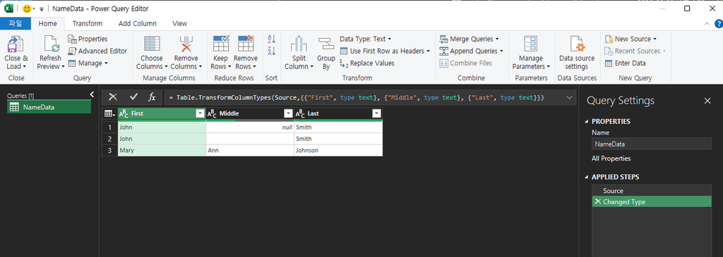
    A column that appears empty at a glance in Power Query can hold either null or "" (an empty string). In this project’s observed preview, null appeared in italics while an empty string appeared as a plain blank cell. Functions like Text.Combine treat the two differently, and mixing them up silently produces wrong results — not an error.

    Applies to: Power Query / Get & Transform in all current Excel versions (Excel for Microsoft 365, Excel 2024, Excel 2021, Excel 2019, Excel 2016) and Power BI, since the M language and its functions behave the same way across these hosts.

    The Problem: A Middle Name Column

    Take a simple “combine three name columns into one” task — First, Middle, Last — joined with Text.Combine and a space separator:

    Text.Combine({[First], [Middle], [Last]}, " ")

    For most rows this works exactly as expected. But this project directly reproduced a case where two rows that both “look” like they have no middle name produce different results:

    • A row where Middle is null: Text.Combine skips it entirely. Result: “John Smith” (one space between the names, as expected).
    • A row where Middle is "" (empty string, not null): Text.Combine does not skip it — it still inserts a separator on each side of the empty value. Result: “Jane Doe” — two spaces between “Jane” and “Doe”, not one.
    Power Query data preview showing null displayed in italics versus an empty string

    This is exactly the kind of bug that passes a quick visual check and then breaks something downstream, like a text match or a fixed-width export — the extra space is easy to miss just by looking at the result, but it’s really there and will affect anything that compares the text exactly or counts characters.

    Why This Happens

    Text.Combine joins a list of text values into one, and it treats null as “no value to contribute” — it does not add a separator for a null entry. An empty string, on the other hand, is a real value (a zero-length piece of text), so Text.Combine treats it as a legitimate entry that still gets a separator placed around it, even though the value itself contributes nothing visible.

    Text.Combine skipping a null value and producing a single space between names, compared with an empty string producing a double space

    It’s worth noting that Excel’s own Go To Special > Blanks command draws a related but not identical distinction: it selects genuinely empty cells, not cells that merely display as blank because a formula returned “”. The underlying lesson is the same one this article is about — don’t assume “looks empty” means “is empty” — but Excel’s blank cell and Power Query’s null are not literally the same data type, and Go To Special’s cell-selection behavior isn’t run through the same code as Text.Combine. Treat the comparison as a useful reminder to check, not as proof that the two features work identically.

    How to Tell Them Apart

    In the Power Query editor, null values are displayed in italics; empty strings display as a blank cell without italics. This is a visual cue you can check directly in the data preview — it’s easy to miss if you’re scanning quickly, but it’s there.

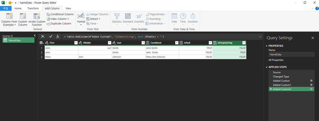
    To check programmatically instead of relying on the visual difference, add flag columns with Table.AddColumn. As a full Advanced Editor step sequence, chained so each step references the previous one:

    IsNull = Table.AddColumn(Source, "IsNull", each [Middle] = null, type logical),
    IsEmptyString = Table.AddColumn(IsNull, "IsEmptyString", each [Middle] = "", type logical)

    This adds a column that’s TRUE only for a genuine null, and a separate column that’s TRUE only for an empty string, so you can see row by row which rows actually have which value.

    Table.AddColumn flag columns distinguishing null from empty string row by row

    If you’re building this through the UI instead of the Advanced Editor, use Add Column > Custom Column twice — once per flag. In the Custom Column dialog, you don’t paste the Table.AddColumn(…) wrapper; you only enter the expression after each, i.e. [Middle] = null for the first column and [Middle] = "" for the second. Power Query generates the surrounding Table.AddColumn step for you.

    How to Fix It

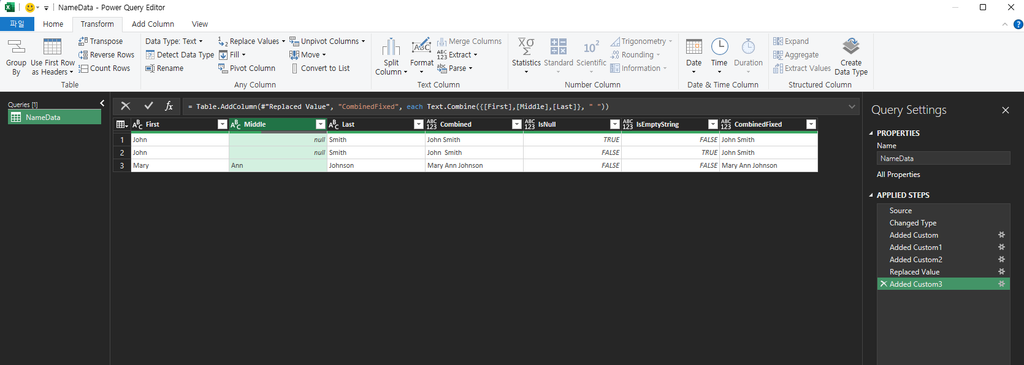
    If you want both null and "" treated the same way (skipped, not contributing a stray separator), normalize one to the other before combining — for example, replace empty strings with null first:

    Table.ReplaceValue(Source, "", null, Replacer.ReplaceValue, {"Middle"})

    After this step, every “no middle name” row is a genuine null, and Text.Combine will skip all of them consistently, regardless of whether the original data used null or “” to represent “nothing here.” For how null and empty-string keys behave when you remove duplicates, see our guide on Power Query Remove Duplicates.

    One practical note from testing this: Power Query columns are computed once, at the step where they’re added, not live-recalculated. If you already have a Text.Combine step earlier in your query, adding Table.ReplaceValue after it will not retroactively fix that column’s existing output. Put the Table.ReplaceValue step before your Text.Combine step, or add a fresh Text.Combine column after the fix, to see the corrected result.

    Table.ReplaceValue normalizing empty strings to null before combining text

    One-line Summary

    Text.Combine skips null values but not empty strings (“”) — a null “no value” is invisible to it, while an empty string is a real, zero-length value that still gets a separator placed around it, producing an extra space that’s easy to miss on a visual check. Use Table.AddColumn with each [Column] = null / each [Column] = “” to check which rows actually have which value, and normalize “” to null with Table.ReplaceValue before combining if you need consistent behavior.

    Sources

    • Text.Combine — Microsoft Learn (Power Query M reference). Backs the general syntax and purpose of Text.Combine (joining a list of text values with a separator).
    • The specific behavior difference — Text.Combine skipping null but not skipping “”, including the exact resulting text for both cases — was directly reproduced by this project in Power Query, including a dedicated fixture and 5 screenshots. This distinction is not explicitly spelled out in the Text.Combine reference page itself; it is project-verified behavior, not a direct quote from official documentation.
  • Split Comma-Separated Values into Rows in Excel (TEXTSPLIT vs Power Query)

    A single cell like Apple, Banana, Cherry sometimes needs to become three separate rows instead of three separate columns — for example, to make each value filterable, sortable, or usable in a pivot table. Excel has two ways to do this, and which one you can use depends on your Excel version.

    Applies to: Excel for Microsoft 365 and Excel 2024 (TEXTSPLIT, native row-splitting); Excel 2021, 2019, and 2016 (Power Query fallback — TEXTSPLIT is not available).

    Method 1: TEXTSPLIT (Microsoft 365 / Excel 2024 only)

    TEXTSPLIT splits text using a delimiter you specify, and it can split into rows, not just columns, by passing the delimiter as the row_delimiter argument instead of the default col_delimiter:

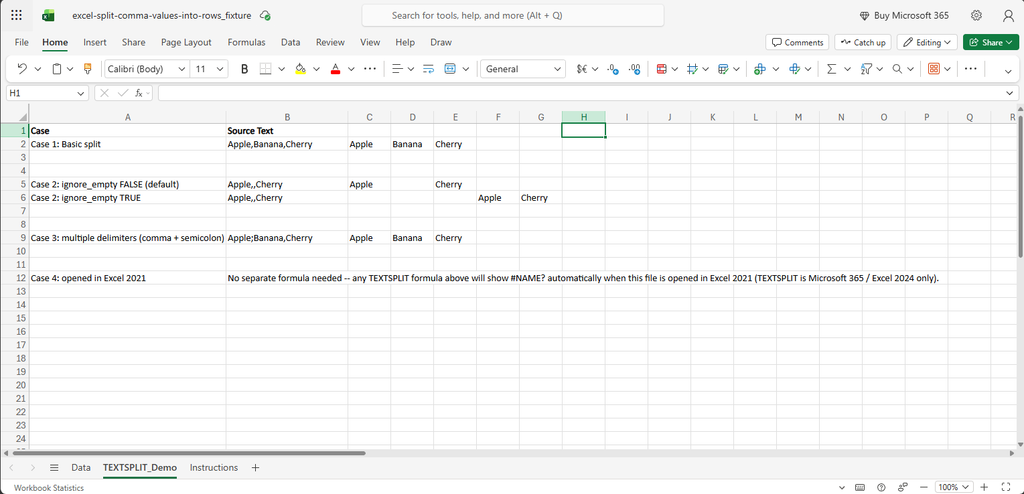
    =TEXTSPLIT(A2, , ",")

    This splits the text in A2 on commas and spills the results downward into separate rows starting at the formula’s cell (the blank argument skips col_delimiter so only row_delimiter is used).

    Microsoft documents three behaviors of TEXTSPLIT that matter for this task:

    • row_delimiter: the argument that controls splitting into rows, as used above.
    • ignore_empty: when set to TRUE, consecutive delimiters (for example, Apple,,Cherry) do not produce a blank row between values. The default is FALSE, which does produce blank entries for empty splits.
    • Multiple delimiters: row_delimiter accepts an array of delimiters (for example, {“,”, “;”}), so a column mixing comma- and semicolon-separated values can be split with one formula.
    TEXTSPLIT formula splitting comma-separated values into rows in Excel, including ignore_empty and multiple-delimiter cases

    Because the formula spills, do not type anything into the cells below it — TEXTSPLIT needs that space to place the split results, and existing content there will cause a #SPILL! error.

    Why TEXTSPLIT Might Not Work For You

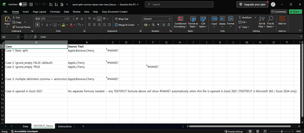
    TEXTSPLIT is a newer dynamic-array function. This project directly reproduced the following in Excel 2021: entering a TEXTSPLIT formula returns #NAME? — Excel 2021 does not recognize the function name at all, across every delimiter/blank/multiple-delimiter case tested. This matches Microsoft’s own version scoping for the function, which lists Microsoft 365 and Excel 2024 as the supported versions.

    TEXTSPLIT formula returning #NAME? error in Excel 2021, which does not support the function

    If you see #NAME? after typing a TEXTSPLIT formula, that is very likely the cause — not a typo in the formula. Another function that returned #NAME? in our Excel 2021 is TEXTBEFORE; see our guide on extracting text before or after a character.

    Method 2: Power Query (Excel 2021, 2019, 2016)

    Power Query’s Split Column by Delimiter, using the Rows option instead of the default Columns option, does the same job on older Excel versions:

    1. Select the column you want to split.
    2. Go to Data > Get & Transform > From Table/Range (or open the query in Power Query Editor if the data is already a query).
    3. Right-click the column, choose Split Column > By Delimiter.
    4. Choose your delimiter (Comma, Semicolon, or Custom).
    5. Under Split into, choose Rows instead of the default Columns.
    6. Click OK, then Close & Load.
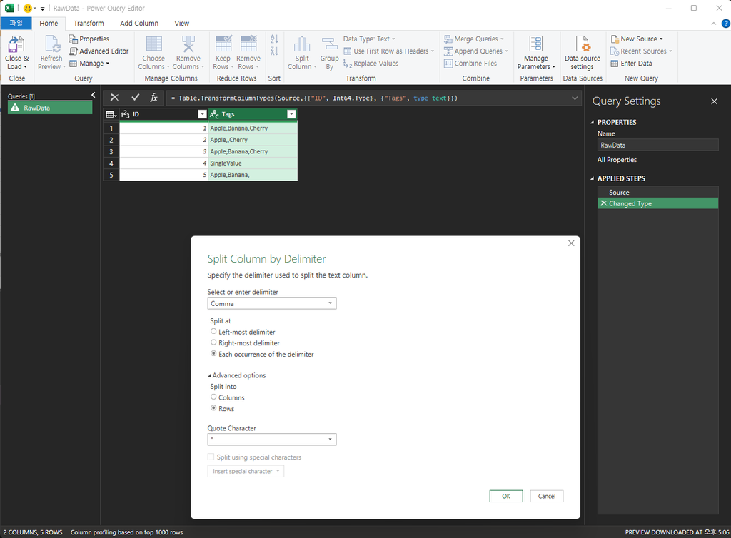
    Power Query Split Column by Delimiter dialog with Rows selected

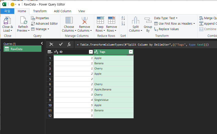
    The Split Column by Delimiter dialog takes a single delimiter per step (Comma, Semicolon, or one Custom value you type in) — it does not have TEXTSPLIT’s array-of-delimiters argument for mixing delimiter types in one pass. This project confirmed the result directly: splitting a column that mixes delimiters (for example Apple;Banana,Cherry) by comma only splits on the comma — the semicolon-joined portion (Apple;Banana) stays together as a single value. To fully split mixed-delimiter data, run the Split Column step again on the result (once per delimiter type), or normalize all delimiters to one character first (for example with a Find & Replace step) before splitting.

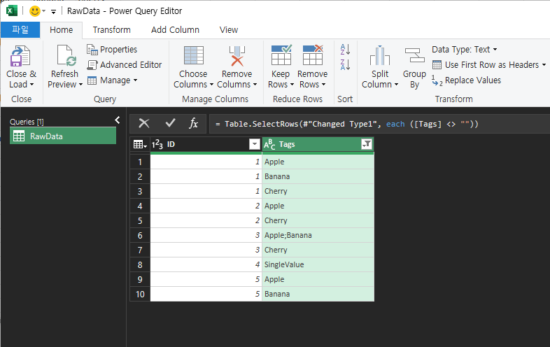
    This project confirmed how the split-into-rows step behaves on consecutive delimiters (for example, Apple,,Cherry): unlike TEXTSPLIT’s ignore_empty argument, Power Query has no built-in option to skip blank results — splitting produces a literal blank row wherever two delimiters are adjacent (or a delimiter is at the start/end of the text). To remove them, filter the split column afterward: click the column’s filter arrow and uncheck (blank), or use Home > Remove Rows > Remove Blank Rows.

    Power Query result showing comma-separated values split into individual rows, including a blank row from consecutive delimiters
    Power Query filter step removing blank rows created by consecutive delimiters

    Which Method Should You Use?

    TEXTSPLITPower Query
    Excel versionMicrosoft 365, Excel 2024 only2016, 2019, 2021, 2024, Microsoft 365 (all versions)
    Result typeFormula (recalculates automatically when source cell changes)Query (needs “Refresh” to pick up source changes)
    Skips blank splitsYes, via ignore_empty argumentNo built-in option — produces a blank row; filter it out afterward
    Multiple delimitersYes, via a delimiter arrayNo — one delimiter per step; run the split again per delimiter type, or normalize first

    If you’re on Microsoft 365 or Excel 2024, TEXTSPLIT is simpler for a one-off, self-updating formula. If you’re on an older version, or you’re already building a Power Query pipeline for other cleanup steps, the Power Query method keeps everything in one place and doesn’t depend on a specific Excel version.

    One-line Summary

    Use TEXTSPLIT(cell, , delimiter) to split values into rows on Microsoft 365 or Excel 2024. On Excel 2021, 2019, or 2016 — where TEXTSPLIT returns #NAME? — use Power Query’s Split Column > By Delimiter, choosing Rows instead of Columns. Power Query produces a blank row for consecutive delimiters (filter it out afterward) and splits on only one delimiter per step (run it again per delimiter type for mixed data) — both confirmed by this project’s own reproduction, not just documentation.

    Sources

    • TEXTSPLIT function — Microsoft Support. Backs the row_delimiter, ignore_empty, and multiple-delimiter-array behavior described in Method 1, and the Microsoft 365 / Excel 2024 version scoping.
    • Split a column of text (Power Query) — Microsoft Support. Backs the Split Column by Delimiter steps in Method 2, including the Rows-vs-Columns choice.
    • The specific finding that TEXTSPLIT returns #NAME? in Excel 2021 was independently reproduced by this project in real Excel 2021 across all tested delimiter/blank/multiple-delimiter cases. Power Query’s blank-row and multi-delimiter behavior for the Split Column by Delimiter step was also independently reproduced by this project (fixture and screenshots): splitting produces a literal blank row for consecutive delimiters with no built-in skip option, and splits on only the one delimiter chosen per step.
  • Power Query Remove Duplicates: Latest Row, Ties & Nulls

    Excel’s built-in Data > Remove Duplicates command always keeps the first row it encounters for each duplicate key and deletes the rest. That’s fine when “first” is the row you actually want to keep. It’s a problem when you need the latest record per customer, an ID column with occasional blanks, or a tie between two rows updated on the same day.

    Power Query handles all of these, but it needs to be told explicitly which row to keep — it does not have a single “remove duplicates, keep the newest” button. This guide builds that logic step by step, covering the edge cases that break a naive approach.

    Applies to: Excel for Microsoft 365, Excel 2024, Excel 2021, Excel 2019, and Excel 2016 (Power Query / Get & Transform is available in all of these).

    Why Not Just Use Remove Duplicates?

    Microsoft documents that Excel’s Remove Duplicates command keeps the first occurrence of a duplicate and deletes the rest of the rows that match on the columns you selected as the comparison key. There is no option to control which occurrence survives — it’s always the first one in sheet order.

    If your data isn’t already sorted so that the row you want is first, Remove Duplicates will keep the wrong row. And once it deletes a row, that’s it — there’s no audit trail showing what was removed or why.

    Power Query solves both problems: you can define exactly which row should win, and the query itself documents the logic (it’s a repeatable set of steps, not a one-time deletion). If you only need to find duplicate or missing items without deleting anything, see our guide on comparing two lists in Excel.

    The Building Block: Group and Pick One Row

    The core pattern used throughout this guide is group by the key, then pick one row per group using Table.Group with a custom aggregation:

    Table.Group(Source, {"CustomerID"},
      {{"Chosen", each Table.First(Table.Sort(_, {{"SortColumn", Order.Descending}})), type record}}
    )

    Read this as: “group all rows by CustomerID; within each group, sort by SortColumn descending, and keep only the first row of that sorted group.” Change what you sort by, and you change which row survives.

    Table.Group with this aggregation produces a table with one column per grouping key plus a Chosen column holding a record (the whole winning row, packaged as one value) — not yet a normal flat table. Every case below needs one more step to turn that back into real columns:

    Table.ExpandRecordColumn(
        GroupedResult,
        "Chosen",
        List.Difference(Table.ColumnNames(Source), {"CustomerID"})
    )

    GroupedResult already has a CustomerID column (the grouping key), and the Chosen record also contains a CustomerID field (it’s the whole original row). Expanding all of Chosen‘s fields — including CustomerID again — would try to create a second CustomerID column and fail. List.Difference removes the key column(s) from the list of fields to expand, so only the non-key fields come out of Chosen, and the existing CustomerID column from the grouping step is kept as-is.

    Each case in this guide produces a grouped-and-sorted table exactly like GroupedResult above; add this expand step as the final step in every case to get the actual result table. For Case 3, which groups on a composite key, replace the last argument with List.Difference(Table.ColumnNames(Source), {"CustomerID", "OrderDate"}) instead.

    Case 1: Basic Duplicate Key

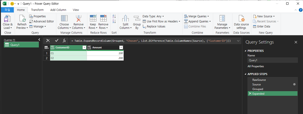
    If you just need one row per CustomerID and don’t care which one, group by the key and take the first row of each group as-is (no sort needed, or sort by whatever column reflects your preferred tie-break):

    Table.Group(Source, {"CustomerID"}, {{"Chosen", each Table.First(_), type record}})

    This is the Power Query equivalent of Remove Duplicates on a single column — except you can see and modify the logic later. If you only need a list of the distinct values, and your Excel does not have UNIQUE(), see our guide on getting unique values in Excel 2019 and 2016.

    Power Query Editor result with one row per CustomerID: C1 with Amount 100 and C2 with Amount 200, after the Grouped and Expanded steps

    Case 2: Keep the Latest Row Per ID

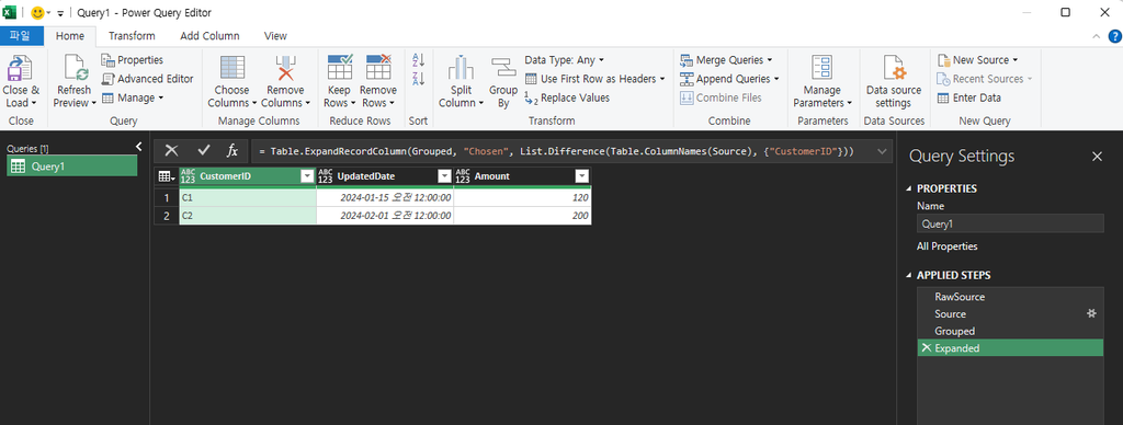
    To keep the most recently updated record per customer, sort by the date column descending before taking the first row of each group:

    Table.Group(Source, {"CustomerID"},
      {{"Chosen", each Table.First(Table.Sort(_, {{"UpdatedDate", Order.Descending}})), type record}}
    )

    This is the pattern Remove Duplicates cannot express — it has no concept of “sort within each duplicate group first.”

    Power Query Editor result with CustomerID, UpdatedDate and Amount: C1 dated 2024-01-15 with 120 and C2 dated 2024-02-01 with 200

    Case 3: Two-Column (Composite) Key

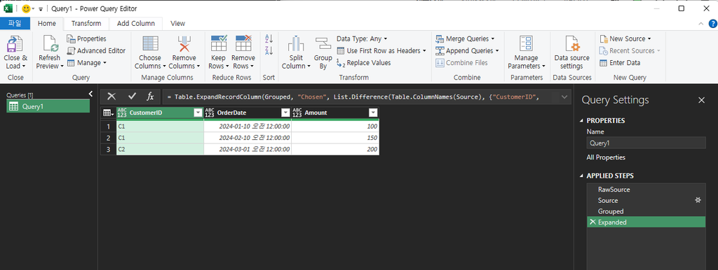
    Some data doesn’t have a single unique identifier — a duplicate is only a duplicate if two columns match together (for example, CustomerID and OrderDate). Group on both columns by passing a list of column names:

    Table.Group(Source, {"CustomerID", "OrderDate"},
      {{"Chosen", each Table.First(_), type record}}
    )

    Grouping on the wrong single column here (just CustomerID, for instance) would collapse legitimately different orders from the same customer into one row — a correctness bug, not a cleanup.

    Power Query Editor result with CustomerID, OrderDate and Amount: C1 on 2024-01-10 with 100, C1 on 2024-02-10 with 150, and C2 on 2024-03-01 with 200

    Case 4: Blank or Null Keys

    Rows with a blank or null key deserve a deliberate decision, not an accident. Table.Group treats null as its own group value — every row with a null key gets grouped together and only one of them survives, which silently deletes the others if you’re not expecting it.

    Before grouping, decide explicitly:

    • Decide whether null and "" (empty string) both count as “missing” for this key. They are not the same value — Table.Group treats null as its own group and an empty-string key as a different group from null — so a filter written as <> null will still group every "" key together and silently keep only one of those rows. If both should be treated as missing, filter both explicitly: Table.SelectRows(Source, each [CustomerID] <> null and [CustomerID] <> "").
    • If blank-key rows are genuinely bad data, filter them out first (using the null-and-"" check above, as appropriate to your data) and handle them separately.
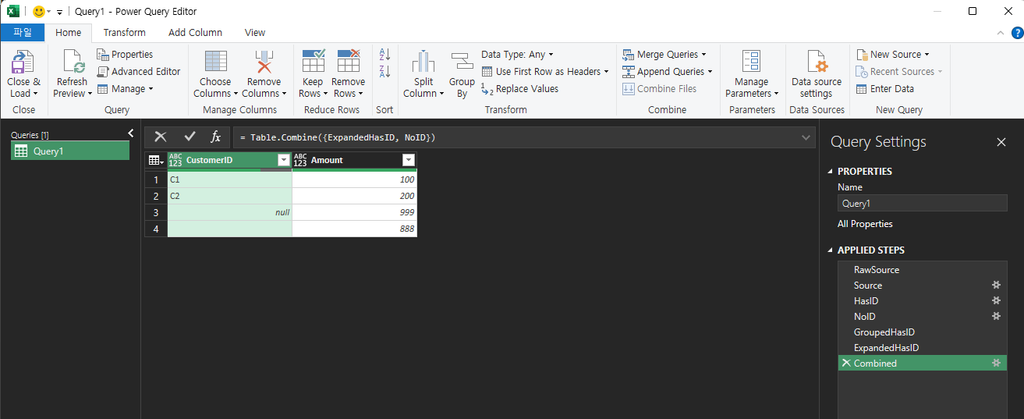
    • If blank-key rows are all real, distinct records that happen to be missing an ID, do not group them with the rest — route them around the deduplication step entirely (for example, split the table into “has ID” and “no ID” with Table.SelectRows on the negated condition, deduplicate only the “has ID” side, then combine the results back with Table.Combine).

    The mistake this case guards against is exactly the same shape as the null-vs-empty-string distinction documented elsewhere for this project: Power Query does not treat every “missing” value the same way depending on how it got there, so blank keys need an explicit rule — one that names both null and "" — instead of being left to fall through the default grouping behavior.

    For a closer look at the difference, see our guide on null and empty string in Power Query.

    Power Query Editor with a Combined step using Table.Combine and four rows: C1 100, C2 200, a null ID with 999, and a blank-looking ID with 888

    Case 5: Same-Date Ties

    Sorting by date breaks most duplicates, but two rows can share the exact same date. Sorting by date alone leaves the outcome ambiguous — Power Query will pick a row, but which one depends on the stability of the sort, not a rule you chose.

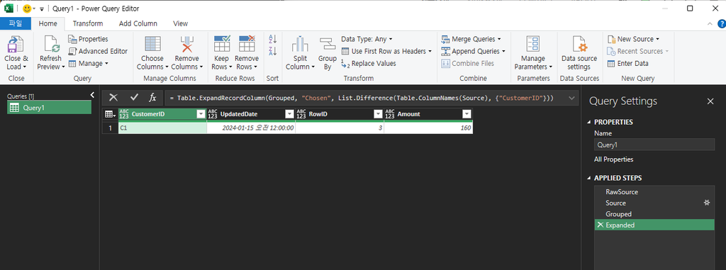
    Add a second, deterministic sort key as a tiebreaker. Starting from the UpdatedDate column already used in Case 2, sort by date descending first, and add a row identifier as the second sort key to decide any tie:

    Table.Group(Source, {"CustomerID"},
      {{"Chosen", each Table.First(Table.Sort(_, {
          {"UpdatedDate", Order.Descending},
          {"RowID", Order.Descending}
        })), type record}}
    )

    When two rows tie on UpdatedDate, the second sort key (RowID descending) decides the winner. Whatever you choose as the tiebreaker — a row ID, an import timestamp, a secondary sequence number — the important part is that it’s a column that is never itself tied, so the result is reproducible every time you refresh the query.

    This pattern assumes every row has a real date. The next case (null dates) shows what to do when that’s not true, and how the tie-break code above needs to change once you’ve handled it.

    Power Query Editor result with a single row: C1, UpdatedDate 2024-01-15, RowID 3 and Amount 160

    Case 6: Null Dates

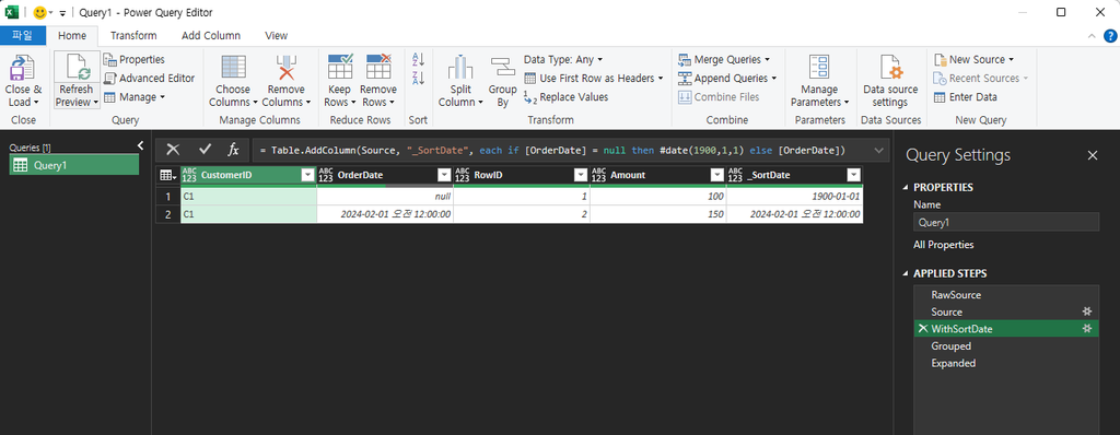
    A null date can’t be compared or sorted the normal way, and it will otherwise sort inconsistently against real dates. This project’s reproduction handled it by substituting a fixed, clearly-out-of-range placeholder date for null before sorting — for example, replacing null with 1900-01-01 in a helper column (here called _SortDate) so every row has a real, sortable value:

    _SortDate = if [OrderDate] = null then #date(1900,1,1) else [OrderDate]

    This guarantees rows with a genuinely missing date always sort as the oldest record for that customer (so a row with real data wins the “keep latest” comparison), rather than causing an error or an unpredictable sort position.

    Combining this with Case 5’s tie-break: once you have the _SortDate helper column, use it in place of UpdatedDate in the Case 5 pattern, so the tie-break is safe against both same-date ties and null dates at once. This project’s own live-test reproduction confirmed the following combined pattern actually executes and resolves ties predictably:

    Table.Group(WithSortDate, {"CustomerID"},
      {{"Chosen", each Table.First(Table.Sort(_, {
          {"_SortDate", Order.Descending},
          {"RowID", Order.Descending}
        })), type record}}
    )

    WithSortDate here is the table after the _SortDate helper column from this case has been added (for example, via Table.AddColumn(Source, "_SortDate", each if [OrderDate] = null then #date(1900,1,1) else [OrderDate])). This is the version to use in practice whenever your data can have both same-date ties and null dates, which is the common case.

    Power Query Editor with a WithSortDate step adding a _SortDate column: the C1 row with a null OrderDate gets 1900-01-01 and the 2024-02-01 row keeps its date

    Case 7: Query Folding

    Query folding is Power Query’s ability to push transformation steps back to the data source (a SQL database, for example) instead of running them locally. It matters here because if a step folds, you’re trusting the source system’s engine to execute your logic instead of Power Query’s own engine — and not every source folds every step the same way.

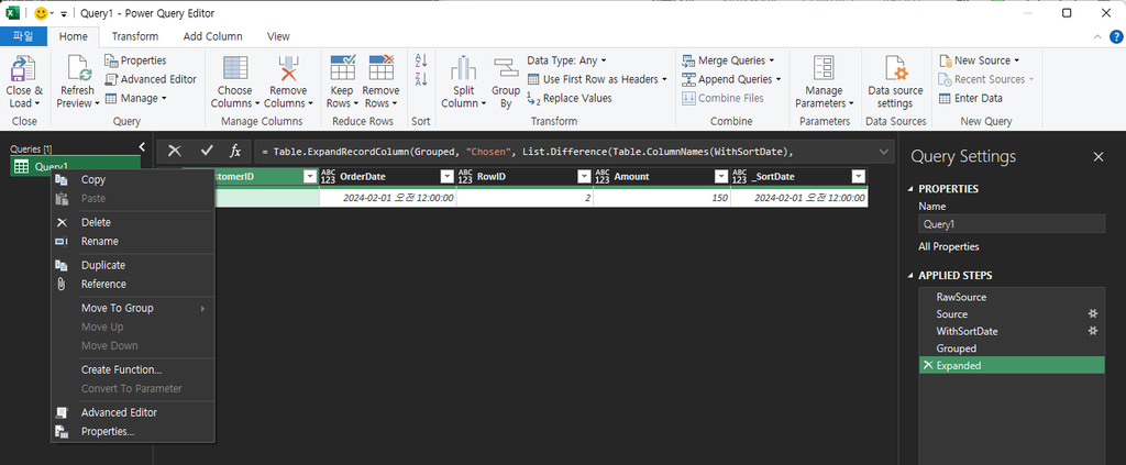
    For data that starts inside the workbook itself (Excel.CurrentWorkbook()), query folding does not apply — an in-workbook table is not a foldable source, so this concern is not applicable for the fixture and workflow described in this article. If your source is a database instead of a workbook table, check whether your grouping and sorting steps still fold as expected before relying on this pattern at scale, since Microsoft documents that Table.Distinct in particular does not generally guarantee which duplicate row survives once folding and query-plan optimization are involved.

    Power Query Editor with the right-click menu open on Query1, listing Copy, Delete, Rename, Duplicate, Reference, Advanced Editor and Properties, with no View Native Query entry

    Case 8: Making the Result Deterministic

    Pulling the cases above together, “deterministic” here means: given the same input data, the query produces the exact same output every time it’s refreshed — no dependence on the order rows happen to appear in the source, and no silent tie-breaking left to chance.

    That requires, in order:

    1. A defined key (single column or composite — Cases 1 and 3).
    2. A defined primary sort for “which row wins” (Case 2).
    3. A defined, never-tied secondary sort for ties (Case 5).
    4. A defined substitution for values that can’t sort normally, like null dates (Case 6).
    5. An explicit decision for rows with a blank/null key, made before grouping rather than left to fall through it (Case 4).

    Skip any one of these and the query can still run — it just won’t be guaranteed to give you the same answer twice.

    Excel sheet Query1 loaded with one row, C1 with OrderDate 2024-02-01, RowID 2, Amount 150 and a _SortDate column, and the Queries pane showing 1 row loaded

    One-line Summary

    Excel’s Remove Duplicates always keeps the first row and gives you no control over which one that is. Power Query’s Table.Group + Table.Sort + Table.First pattern lets you define exactly which row wins — by recency, by a composite key, and with an explicit, never-tied tiebreaker for same-date rows — as long as you also decide up front what happens to blank keys and null dates instead of leaving them to the default behavior.

    Sources